 Factor(T)
 1, then T is height-balanced.


The time required to locate a value or discover that it is not present in a binary search tree is dependent on the depth of the tree. It is customary to refer to the depth as height and talk about height-balanced binary trees, a denotation due to the developers of efficient management techniques that control the shape of ordered binary trees. Such trees are called AVL trees after Adelson-Velskii and Landis [ADELSON, 1962.]
The height of tree T is h(T). For node p, h(p) is the height of the subtree rooted at p.
The balance factor of binary tree T with subtrees L rooted at its left child and R rooted at its right child is Factor(T) = h(L) - h(R). This definition extends to any node of a binary tree. If T is an empty tree, Factor(T) = 0.
If  Factor(T)
 1, then T is height-balanced.
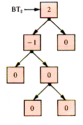
The nodes of BT8, in Figure R.1 are tagged with their balance factors:
Exercise ER.1 and Problem PR.1 are appropriate at this point.
Given a binary tree bt and a value v, one position at which v may be inserted to retain the order property is determined by NodeSpot and inserted by InsertNode (section 8.5.2). The result is not the only BST with the values it contains. The goal of AVL management is to rearrange bt after the addition of each value so that it is both height-balanced and a BST. There are a number of cases to consider.
A general binary tree T is of the form shown in Figure R.2 .
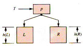
If h(L) = h(R), then Factor(T) = 0 and the addition of one node to form a new binary tree T' may (or may not) change the balance factor of the root node p to  1, whence T' is still balanced at the node p. Balancing within L or R may be necessary. Note, for example, that a child added to the leftmost leaf node of BT8, would not change the balance of the root node, but an addition to other leaves would do so. Two rightmost additions will leave the root node balanced but the balance factor of the rightmost node of BT8, would change to + 2.
Exercise ER.2 is appropriate at this point.
If h(L) - h(R) = 1, then the addition of a node to R will leave the resulting Factor(p) either 0 or 1 for the root node p, still balanced. If, however, the new tree T' is formed by adding a node to L, the result can be that Factor(p) = 2 unless an adjustment is made. A suitable adjustment switches some of the nodes of L to the right subtree without violating the order property. In that case, p is said to act as a pivot.
Suppose an addition is made to the subtree L, rooted at node Lroot. If the left and right subtrees of Lroot are LL and LR, respectively, then no unbalance is created by an addition unless the height of one of these subtrees is h(R) and the addition is to that subtree and increases its height. Figure R.3 is a model of T.
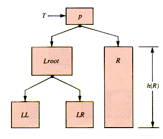
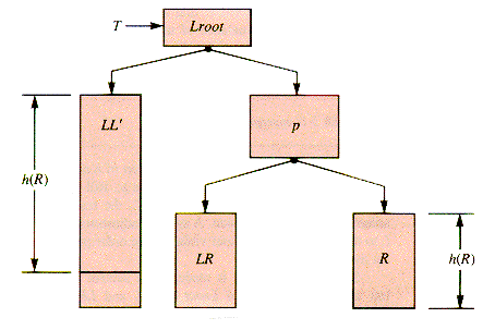
If the addition increases h(LL) to h(R) + 1, T can be restructured without violating the BST property by using p as a pivot, as shown in Figure R.4. If h(L) - h(R) = - 1 and the addition is at the right in the subtree RR (the analog of LL), the pivot in the opposite direction that may be necessary is symmetric.
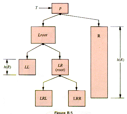
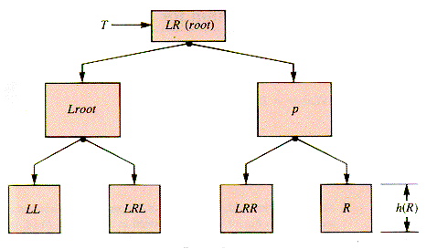
A second case occurs when h(LR) = h(R) and an addition is made to LR that causes h(LR) to become h(R) + 1, whence h(Lroot) becomes h(R) + 2. The pivot above will not balance the tree and so one level deeper is involved, as Figure R.5 illustrates. This can be rearranged without violating the BST property by using p as a pivot, as in Figure R.6. The new T' will be balanced if either h(LRR) or h(LRL) is increased by the added node. The symmetric right subtree case for which Factor(T) = - 1 may also occur and be dealt with by a symmetric pivot.
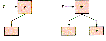
A special case is required for the addition of a node nn to the non-null child of a two-node binary tree. Figure R.7 shows how the left version of this pivot is modeled.
It is important to realize that "root node" generally refers to the root of a subtree, and that pivoting is carried out as deep in the tree as possible.
Exercises ER.3 and ER.4 are appropriate at this point.
It is convenient to include a field for the balance factor in the nodes of an AVL tree:
AVLnode = RECORD
Value : {value type
Left :AVLnode
Right :AVLnode
Factor : INTEGER
END
As a node is inserted, the location of the parent of the inserted node and the closest ancestor with Factor > 0, are retained in Parent and Pivot, respectively.
An AVL tree is a BST, and so InsertNode (section 8.5.2) can be used to insert a node p in the tree T. However, it is necessary to modify NodeSpot (section 8.5.2) in order to retain a pointer, Pivot, to the closest ancestor of the new node with nonzero balance factor and its immediate ancestor Parent. This can be done by initializing Pivot to T and Parent to NIL and adding the statement
if p.Factor
0
then Pivotp
ParentPred
endif
as the first statement within the while loop in NodeSpot.
The insertion algorithm becomes:
procedure AVLinsert(nn,T)
if Empty(T)
then Tnn
nn.Factor
0
return
endif
NodeSpot(T,nn.Value,Trio,p,Pred,Pivot,Parent)
InsertNode(T,nn,Pred,Trio)
{small-tree cases are
if T.Right = NIL {treated separately
then PairLeft
return
endif
if T.Left = NIL
then PairRight
return
endif
{change factors between Pivot and
NewFactors {nn, and determine the apparent
{change to Pivot  .Factor, PF
if Pivot.Factor = 0
then Pivot.Factor
PF
return
endif
if Pivot.Factor + PF = 0
then Pivot.Factor = 0
return
endif
if PF < 0
then LeftPivot
else RightPivot
endif
end {AVLinsert
procedure NewFactors
pPivot
vnn
.Value
if p.Value < v
then pp
.Right
PF-1
else pp
.Left
PF+1
endif
Hubp {the first node between Pivot and nn
while pnn do
if p.Factor < v
then p.Factor
-1
pp
.Right
else p.Factor
+1
pp
.Left
endif
endwhile
end {NewFactors
procedure LeftPivotd
if Hub.Factor = 1 {do a simple rotation of Hub
then Pivot.Left
Hub
.Right
Hub.Right
Pivot
Pivot.Factor
Hub
.Factor
Hub.Factor
0
if nn.Value < Parent
.Value
then Parent.Left
Hub
else Parent.Right
Hub
endif
return
endif
{do a deeper rotation
CogHub
.Left
CogLeftCog
.Left
CogRightCog
.Right
Hub.Right
CogLeft
Pivot.Left
CogRight
Cog.Left
Hub
Cog.Right
Pivot
case of Cog.Factor
+1 : Pivot.Factor
-1
Hub.Factor
0
-1 : Pivot.Factor
0
Hub.Factor
+1
else: Pivot.Factor
0
Hub.Factor
0
endcase
Cog.Factor
0
if nn.Value < Parent
.Value
then Parent.Left
Cog
else Parent.Right
Cog
endif
end {LeftPivot
RightPivot is similar.
A PairLeft procedure can be implemented like this:
procedure PairLeft
T.Left
NIL
if Trio = 1
then Pred.Right
T
TPred
else nn.Right
T
nn.Left
Pred
Pred.Right
NIL
Tnn
endif
T.Factor
0
end {PairLeftPairRight is similar.
Deletion from an AVL tree requires modification of CutValue (section 8.5.2) to determine Parent and Pivot, and the rebalance operation must proceed up the tree. It is common to forego deletion entirely; inactive nodes may be so marked or simply ignored.
Exercises immediate applications of the text material
ER.1 Calculate the balance factors for all of the binary trees in Chapter 8.
ER.2 Trace the effects of adding two nodes to BT8 at every possible combination of positions.
ER.3 Suppose that the days of the week are used to form an AVL tree by adding them one at a time to an empty tree. Diagram the stages of the tree when they are added in the reverse order: Saturday, Friday, . . ., Sunday.
ER.4 Form an AVL tree from the sequence: 1 3 5 7 9 11 8 6 14 by adding them one at a time. They are to be filed in nondecreasing order. Then repeat for the AVL tree that keeps them in nonincreasing order.
Problem not immediate, but not a major extension of the text
PR.1 Design a procedure to calculate balance factors for an arbitrary binary tree.
Project for fun; for serious students
PJR.1 Write a program that creates an AVL tree by insertion and displays it.
Problem
Project