The simplest way to imitate unpredictable variation is the generation of pseudorandom numbers. A random variable x, 0 < x < 1, has the property that any real number in this range is equally likely. A pseudorandom variable r, 0 < r < 1, has values that approximate true randomness in two ways:
The set of values of r is not complete, but there are many of them and no obvious gaps.
The values in the range of r are of approximately equal likelihood.
A great deal of work has been done on developing programs to produce pseudorandom numbers [KNUTH, 1973], and no programmer should be without access to such programs. In some of the exercises a function Rand, available to provide a pseudorandom number on demand, is assumed. Also assumed is a mechanism for reusing the same value or sequence of values produced by it. This assumption is convenient for debugging purposes to isolate the effect of a change in a program, and it provides a way to compare the effect of more than one procedure on the same data. If no other way is available, successive values of Rand may be stored in an array or in a file.
In some languages, notably standard Pascal, the programmer might need to provide a pseudorandom number generator. The subject of generating pseudorandom numbers is too large to pursue here, but one popular algorithm is illustrated in Pascal:
The values of the constants given here work well on a DEC VAX and other machines, but they will not work well in all cases. For example, for a PDP 11/70, Seed is declared externally by
and the constants become:
The function Rand only produces values between 0 and 1. That does not explicitly allow, for example, the random choice of an index for an array declared as a[ - 2 . . 3]. The requisite mapping can be derived with the following steps:
The expression x = D
The expression x =L + D
The expression x = L + (T - L)
The expression INT(L + (T - L)
Consequently, with T = U + 1, INT(L + (U - L + 1)
A set of 10 values, randomly chosen in the range [- 30 . . 30], may be provided in the array e used in the sorting routines in section 1.5 by:
It is not feasible to explore hypothesis testing, confidence intervals, analysis of variance, and so on in this text. That material belongs in a course in statistics. However, the applicability of Rand can be extended enormously by a few additional tools. Some acquaintance with the ideas of probability and statistics is helpful in reading the subsections that follow.
Program PGA.1 is appropriate at this point.
A sample of values from a population determines a (sample) mean that provides an estimate of the mean value of the population, and a (sample)standard deviation that is an estimate of the dispersion of the population. For a sample of size n they can be calculated by:
These measures provide a convenient and significant way to reduce a collection of measurements to two values, but intelligent interpretation then requires knowledge of statistics.
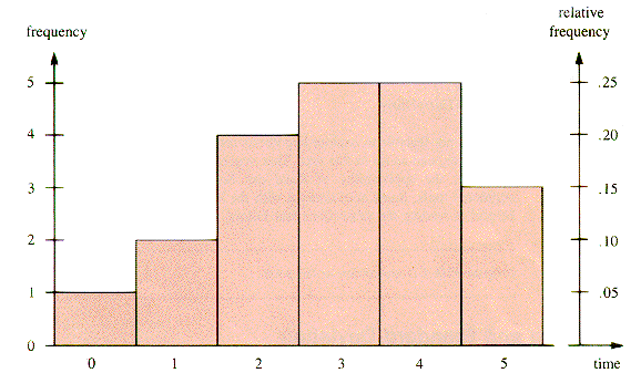
A plot of how many minutes 20 people had to wait in line at the check-out counter of a grocery store might look like the histogram of Figure A.1.
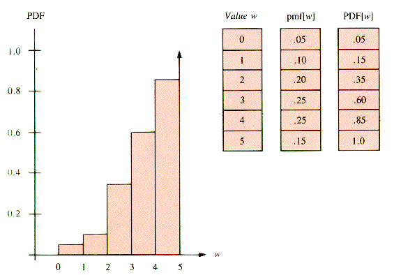
If this sample of size 20 is the only information about waiting time available, then it must provide the model for the probability, P[w], of waiting w minutes. That model is the relative frequency, which is scaled to the right of the histogram. Given that this model is a valid estimate, the relative frequency as a function of time can be accepted as a pmf (probability mass function). The accumulated (summed) values of a pmf are the cumulative probability. The distribution of cumulative probability is called the PDF (Probability Distribution Function). For this example, the PDF is plotted in Figure A.2.
Now suppose that we wish to write a program to process data that have the distribution model derived from the sample. We may provide a random variate, Line, for test data by the following:
Choose a value with Rand, uniformly distributed between 0 and 1. If PDF[w - 1] < Rand
Geometrically, this amounts to drawing the horizontal line from a point on the vertical PDF axis to where it first strikes the stairstep graph and projecting down to a value w. The distribution of Line is that of the pmf (from the histogram), and points may be drawn from this distribution as required.
Values that have the pmf of any discrete PDF may be generated from a table like Figure A.2 in this way, which is called discrete inversion.
Exercise EA.1 and Problem PA.1 are appropriate at this point.
The most-used probability distribution is not discrete as are those discussed in section A.1 but is the normal distribution:
Here,
{Rand is called n times.
In particular, this equation is simplified if n is taken to be 12, in which case:
The z-scores generated in this way can be mapped to a value from a normal distribution by:
A function that returns a value from a normal distribution is:
Note: Some caution must be applied to normal distributions because extreme values can occur, whatever
Program PGA.2 is appropriate at this point.
Arrival times for customers in line at a bank teller's window and for many other arrival and departure processes have neither a uniform distribution like Rand nor a normal distribution like Norm. The arrival times are more likely to form a Poisson Distribution for which the probability that n arrivals have occurred by time t is:
In practice, the time interval between arrivals is more useful. This is called the interarrival time, and it has an exponential distribution. A variate with an exponential distribution may be derived from Rand by
where LOG is the logarithm to the base e (2.718 . . . ). The distribution of values of ia has both mean and standard deviation equal to 1/
Exercises immediate applications of the text material
EA.1 Develop the function Line that will return a value, with the set of such values distributed according to the histogram given in section A.2.
Problems not immediate, but requiring no major extensions of the text material
PA.1 The solutions in a high-school programming contest are timed to the nearest minute. Data from a preliminary contest for the first, "courage-builder," problem came out like this:
Plot the (relative) frequency distribution of this data. Assume that this represents a pmf, and plot the corresponding PDF. What times correspond to the following possible values of Rand?
(a) 0.007134 (c) 0.567321 (e) 0.410022
(b) 0.916528 (d) 0.757505
Programs for trying it out yourself. A program, when written for an interactive system, should display instructions that explain to the user what it does and how to use it. It should provide a graceful way for the user to quit.
PGA.1 Write a program that compares the execution times of SelectionSort, BubbleSort, and InsertionSort for 20 sets of 20 values, generated by the uniform variate, Rand. Calculate the mean and standard deviation for the three execution times.
In a time-sharing system it may not be possible to determine execution times themselves, but it is possible to count statement executions, including those that result from data-determined, conditional branches.
PGA.2 Do PGA.1, except that a normal distribution is to be used for data values, with mean 10 and standard deviation 10. For contrast, also use data already in order and in reverse order.
Projects for fun; for serious students
PJA.1 Extend PGA.1 and PGA.2 to a serious study of SelectionSort, BubbleSort, and InsertionSort for values of n = 8, 16, 32, 64, 128, 512, and 2048. Use uniform, normal, and exponential variates, in-order and reverse-order data sets, and data sets that are somewhat disarranged from in-order in a variety of ways. For example, choose two indices at random from an in-order sequence and switch the values they point to prior to invoking the sort procedure being studied. Calculate means and standard deviations of execution time. If you have statistics in your background, test the hypothesis that the three sorts have equal execution times (under various circumstances).
FUNCTION Random (VAR Seed : INTEGER) : REAL;
CONST Modulus = {65536};Multiplier = {25173};Increment = {13849};BEGIN
Seed : = ((Multiplier * Seed) + Increment) MOD Modulus;
Random : = Seed/Modulus
END {Random};VAR Seed : 0 . . 65535;
Modulus = 32768;
Multiplier = 13077;
Increment = 6925;
 Rand has values in the range 0 < x < D when 0 < Rand < 1, and D > 0.
 Rand has values in the range L < x < L + D.
 Rand has values in the range L < x < T.
 Rand) takes on integer values L, L + 1, . . . , T - 1 when INT is a function that returns the largest integer less than or equal to its argument.
 Rand) has possible values L, L + 1, . . . , U. In particular, INT(- 2 + 6
  Rand will randomly provide in-bounds indices for the array a[ - 2 . . 3].
procedure ThirtyThirty {O(1)for i = 1 to 10 do
e[i]
 - 30 + 61 * Rand
next i
end {ThirtyThirtyA.1 Mean and Standard Deviation

A.2 Frequency Distributions

Figure A.1
 PDF[w], then Line
  w.
w.
Figure A.2
A.3 Normal Distributions

 is the mean value of x, and
  is the standard deviation of its values. The standard normal distribution is defined as the one for which
  = 0 and
  = 1. The relationship given above between z and x defines a map for any normally distributed variable to z-scores, and back again. It is possible to approximate the distribution of z-scores, (the standard normal distribution), by using n values of Rand:

x =
 +
+  z
zfunction Norm(Mu,Sigma) {O(Rand)z
 0
0for i = 1 to 12 do
z
 z + Rand
next i
z
 z - 6
z - 6Norm
 Mu + Sigma * z
end {Norm and
and  may be. Sometimes these values are not physically meaningful: the distribution being modeled differs from a normal distribution by not having them. They are "out of bounds" and must be dealt with by checks within the program.
A.4 Exponential Distributions


 .
.Exercises
Problems
time 1 2 3 4 5 6 7 8 9 10
----------------------------------------
number
of 0 0 0 2 1 5 8 9 7 4
solutions
Programs
Projects


