External storage has been a background theme for all of the structures studied in this book because access to data stored on secondary storage is not done on the same time scale as it is for main storage. Just as important is the massive size of the data files that may be stored externally. The choice of data structure to be used for external storage can be profoundly affected by the need to deal with data sets much too large for main memory. An approach to sorting too much data to retain in main memory is outlined in section 9.2, where it leads to merging and merge- sorting in Part II, sections S and T. Some of the structures that provide access to external data are studied in sections 9.4, 9.5, and 9.6 .
BINARY TREE provides only two children at each node. An obvious generalization is to structure nodes with more than two children. Having more than two children provides quicker access to the deeper levels of the tree. External files are commonly accessed through a directory with such multichild nodes in order to decrease the number of levels used to reach a given number of nodes.
Applications of multiway tree structures include m-way structures in section 9.4, B-trees in section 9.5, 2-3-4 trees in section 9.6 and Part II, section U, and the decision tree of section 9.8 and Part II, section V.
Finally, if a data structure is large, it may be desirable to limit access to part of it--to prune it. That is the theme of (multiway) game trees, section 9.9 and Part II, section W.
9.1 Access by Indirection
One major activity applied to data is sorting, which generally reduces to the sorting of records by key. It is not uncommon to need access to the data in complex records, such as personnel records, by way of more than one key. Sophisticated ways to access data interrelated in complex ways have been developed under the general heading of data bases. A much simpler approach can be of value: indirect sorting.
As a focus, consider an array of student records, a[l . . n], each containing a name and an identification number. If the records are already sorted physically in ID-number order, the names are surely out of alphabetical order, and locating a name becomes an O(n) operation rather than a binary search of O(ln n) cost. It is desirable to provide an ordered appearance for a name search without physically moving the records out of ID-number order.
Any sorting algorithm can be implemented indirectly; and, for contrast, both a direct and an indirect sort with the same algorithm are developed here.
A sorting procedure that compares favorably in practice with those of Chapter 1 is the ShellSort, developed by D. H. Shell. It is O(n2) but may be ten or more times as fast as the other methods are for a few hundred items [KERNIGHAN, 1974]. For large data sets, it is less efficient than HeapSort, but easier to get right. ShellSort acts like BubbleSort except that, as it makes a sweep, it compares a[i] with a[i + Gap], where Gap is initially INT(n/2) instead of 1. If switches occur on a sweep, it resweeps with the same value of Gap; otherwise, it halves Gap and repeats.
To do this procedure by indirection, an array of indices to records in the array must be first created. (Pointers to scattered records would also serve.) The indices are initialized to the initial position of the records:
Immediately after execution of MakeMap, a[i] and a[Map[i]] are identical. However, the indirect sort compares a[Map[i]] to a[Map[j]]; and, if a switch is indicated, it is Map[i] and Map[i] that are switched, not the records themselves. (This technique works for the sorts in Chapter 1 as well.)
After execution of VirtualShell, the records may be displayed in the order determined by their Name fields by:
Exercise E9.1 and problem P9.1 are appropriate at this point.
HEAP is a structure that involves a great deal of data movement when it is managed directly. Actually, it is only the address of data that needs to be provided in heap form, just as a data-set is defined to be fully sorted for a user by an appropriate sequence of addresses. The creation of a heap from the data used for ShellSort follows the procedures in section 8.6 rather closely:
The Name indexed by Map[1] is the top name, whatever its index in a[l . . n].
Finally, it is possible to keep an inverse map. For example, if Track[i] is initialized to i for i = 1,2, . . .,n, then the location of a[j] within the indirect heap, Map, can be followed by adding a small amount of overhead to the switch:
After execution of MakeHeap, the location of a[i] in the (indirect) heap Map is Track[i]. The parent and child nodes and the level of a[i] can all be derived from Track[i] .
Indirection can be a powerful tool for preserving both storage and time, simply because pointers are relatively small.
Exercise E9.2 is appropriate at this point.
Data is stored on disks or tapes in order to preserve it beyond the life of a program execution, but these storage media have been developed with the secondary goal of providing cheap bulk storage. The $2 disk on which this sentence was stored in a portable personal computer holds 195,000 bytes on a side. That is 195,000 characters, or 3,250 sentences like this one. That is enough for a file containing this chapter. The main memory in which such a file would be edited holds an operating system, an editing program, and only a portion of a chapter file. A search through such a file (for misspelled words, perhaps) would require a number of transfers of data between main and secondary storage. Direct access to data in secondary storage may be slower than access to data in the main store of a computing system by a factor of 100 or 1,000 or 10,000. Both their bulk and the time required to access external storage have an impact on the choice of data structures applied to it.
External files with exogenous and/or balanced search-tree directories can combine the speed of main memory with the bulk storage capability of external storage. A common form for such files is that of the m-way trees of section 9.4 and the B-trees of section 9.5, and this is supplemented by material on balanced binary trees in section 8.7; Part II, sections P and R, and Red-Black (2-3-4) trees in section 9.7 and Part II, section U.
One approach to organizing large sorted sequential files that has been applied frequently is similar to the use of index tabs in dictionaries and physical files: quick access is provided to a directory of segments of a file. A key can be efficiently placed within a particular segment, and the segment accessed for further search. This organization is called an indexed-sequential file.
An indexed-sequential file is sorted as a whole. Sorting such a file, or any large file, may need to be done in manageable pieces much smaller than the file itself. The pieces are then merged to form a single file sorted as a whole.
Suppose that two arrays, sorted in nondecreasing order, a[1 . . m] and b[1 . . n], are to be written as a single sorted list on a file. (The output file is taken here to be the standard output file.) This merging operation can be done simply by examining the next item in both arrays and writing the smallest of them:
Variations of StraightMerge can be designed for linked lists, for more efficient operation when one run is larger than another, and as a sorting procedure. Further discussion is to be found in Part II, section S.
When a large file is to be sorted by merging techniques, the efficiency of the complete operation is affected by the size of the sorted segments, called runs. Runs are merged to form larger runs, until there is only one. As the runs increase in size, they cannot be in main memory, and so data is read from two or more files and written onto another in sorted order. The operation of creating runs from sequential files is enhanced by the application of a priority queue. Details are to be found in Part II, section T.
Exercise E9.3 is appropriate at this point.
As noted in Chapter 8, trees and binary trees are not the same structure, but the relationships between the nodes of a tree can be retained in a binary tree. Clearly, any binary tree becomes a tree simply by ignoring the distinction between left child and right child. In that sense, a binary tree is a restricted form of tree. The three common restrictions are:
A link is directional from parent to child.
There are no more than two children per node.
Children of a node are distinguished.
The middle restriction can be restated as:
The degree of each node of a binary tree is no more than 2.
(The degree of a node is the number of links it has to other nodes.) Trees of degree m are used in m-way search trees, in direct analogy with the binary search trees of section 8.5.
Removal of the first two restrictions together with the assumption that a child has but one parent provides a structure that is commonly used to manage sets (see section 9.7). Removal of the last two restrictions provides a family of structures used in decision making and in the analysis of games (see sections 9.8 and 9.9). Removal of all three restrictions creates a graph structure, the subject of Chapter 10.
An increase in the number of children of each node tends to decrease the depth of a tree with a given number of nodes. The depth of a tree determines the maximum number of links that must be traversed in search, insert, or delete operations. Tree depth can be changed by either an insertion or a deletion, which makes it desirable to formulate these operations so that paths from the root to all leaves tend to be the same length. It is possible to balance the root-leaf paths of general tree structures, much like binary trees are balanced in the AVL structure of section 8.7.1. The structures introduced in this chapter provide alternates to AVL trees and randomly formed binary trees, and their balance is a major theme.
Exercise E9.4 and program P9.2 are appropriate at this point.
The mathematical structure of a tree with no more than two children differs in two ways from the computing structure BINARY TREE. One difference is the distinction between left and right subtrees in the binary tree structure. The other difference is that the links in binary trees are directional, and the edges connecting nodes in a mathematical tree are two-way connections. When restriction is made to directional links in a mathematical structure it becomes a directed graph or digraph. A linked list necessarily forms a digraph because links are directional, but when each link is paired with a link in the reverse direction, the pair models an undirected, two-way link.
Figure 9.1 is a valid directed graph. Directed graphs are very general structures, and so general algorithms to traverse them tend to be either more complex or slower than algorithms dealing with structures that have a higher degree of internal structure.
Removal of the one-way linkage restriction on binary trees is well worth considering for any application, particularly if the tree is exogenous. In that case, the Value field of a node record is a pointer to a storage record, and the storage required for the link does not increase the overall storage requirements a great deal. One additional link in each node can be a great help in the management of a structure:
A Visit field is included because it is useful for indicating which subtrees of a node have been explored. A recursive traverse of a tree twt built of TwoWayType nodes does not differ from the recursive traverse of a binary tree, but the extra link simplifies an iterative traverse. (We assume in the following that the parent field of a root node (only) is NIL.) Only minor modification of BTT of section 8.4.1 is needed to walk a tree formed from such nodes.
In the traverse TwoWayVisit that follows, p
TwoWayVisit includes the cases of preorder, inorder, and postorder processing by applying distinct processes at each of the three encounters with a node.
To make a search of a two-way tree for a given value Wanted, it is only necessary to let TwoWayVisit be a function, let processes 2 and 3 be null processes, and let PROCESS1 be:
Exercises E9.5 and E9.6 and problem P9.3 are appropriate at this point.
An immediate generalization in to assume x children and use Child[0] as the parent link:
A very general tree structure, as shown in Figure 9.2, can be built with nodes of the form:
A tree with nodes of this kind is an m-way search tree (MWT) if no more than m of the pointers in ptr may be non-NIL, and suitable restrictions are placed on the keys.
The nodes of an MWT may be generalized by using Value[i] as a pointer to a value record, thereby creating an exogenous search tree. The search tree may then serve as a directory to a file too large to be contained in main (quick-access) memory. Generally, the records themselves reside in auxiliary memory devices, such as disks, as an external file. "Disk" is often used as a synonym for all such devices because it is by far the most common one in use. Any detailed timing analysis of a program that deals with access to disk storage must take into account the difference between fetching and storing on disk and in main memory. Generally, reading from and writing on a file that must be opened and closed by the operating system is many times slower than assignment from or to other variables and needs a separate accounting.
In some implementations, n may be contained as a field of the record, so that the record size may vary. Essentially, the "key" of a node of this type is multivalued; its value is the set of values in the entire array Key, and the search value is found in a node when any of Key[1] . . Key[n] match it. If n is large enough, the search through the n keys of a node may be a binary search, but the dominant factor in the time required for a search often is the number of disk accesses it uses. The number of disk accesses in a search is affected by several factors, such as the shape of the tree and where the key happens to be found in the tree if it is there. One factor that can be controlled by design is whether the key nodes are stored with the records or in a separate directory. An important parameter that can be controlled simply by programming is m, since it determines the minimal depth of the tree.
The formal shape restrictions for the m-way search tree structure follow:
An empty tree is an m-way search tree.
No more than m pointers of the array ptr point to internal nodes.
Key[i] < Key[i + 1] for 1
All key values in ptr[i] are less than Key[i+1] for 0
All key values in ptr[i] are greater than Key[i] for 1
All subtrees ptr[i] for 0
A 3-way search tree file with integer keys 1-9, 12, 15, 18, 21, and 24 with n = 2, m = 3 has the form shown in Figure 9.3. This file can readily be extended to a 3-way file with keys 1-26. Note that it is not particularly well balanced; with no restrictions on balance the extension can be done in a number of ways.
The graph of Faye's Family in Chapter 8 may be taken to indicate family relationships. Additional data, such as the ages of family members would be carried in the value field of records or in records that are the target of a pointer used as a value field. An alternate structure is a 4-way search tree where ages are used as keys (but then descendant information may be carried in some other way), as in Figure 9.4.
Exercise E9.7 is appropriate at this point.
Choices need to be made about including information in the nodes themselves to simplify the algorithms that deal with MWTs. Inclusion of less information in the nodes may complicate the algorithms but save node storage. The choice made here is to include quite a bit of information in the nodes, assuming them to be used as a directory to an external file (external to the MWT-the choice of storage location is an independent decision).
Since m < n is allowed, some keys are inactive and may be so marked. The management of structures involving m-way search trees is eased if the active keys are to the left of the inactive keys. If the nodes are maintained in that form, only m - 1 key slots (m pointers) are needed in the nodes, but one more key slot is usually included because it is very convenient for maintenance of the file. Simplified management routines can be used if three fields are added to the record structure mWayNode:
Active: INTEGER (the number of active keys) If this field is present, there is no need to mark active keys individually.
Up:
UpKey: INTEGER (the key in the parent node that points to the node)
As for all tree structures, random insertion and deletion in m-way search trees tends to randomize their shape and increase the search time in the worst case. To prevent this, MWTs can be balanced, like the AVL trees of section 8.7, and the Red-Black Trees of section 9.6. One form of relatively well-balanced MWT is the B-tree, treated in section 9.5. Management of balanced structures requires sophisticated algorithms and an increase in overhead and should be avoided for relatively small files of perhaps 100 nodes or less.
Search, insertion, and deletion in m-way search trees generally can be readily extracted from the procedures developed in section 9.5 tor B-trees.
Problems P9.4 and P9.5 and program PG9.1 are apropriate at this point.
An m-way search tree (MWT) can be balanced by maintaining the number of children of each node to be between limits. Limits of INT(m/2) and m determine a B-tree. It is convenient to think of external nodes of an MWT as failure nodes.
With this terminology, an m-way search tree is a B-tree of order m if it is empty or:
The root node has at least two children.
All nodes except the root and failure nodes have at least INT(m/2) and no more than m children.
All failure nodes are on the same level. (Each path from root to leaf is the same length.)
Both 3-way1 and 4-way2 fail to qualify as B-trees, but a directory to Faye's Family may be stored in a B-tree as shown in Figure 9.5.
An MWT grows by adding to a node at the deepest level. A node to which an addition is made may split because the number of keys it is to contain has reached m + 1.
Note: It is convenient to allow a B-tree of order m to have m + 1 children temporarily, so that splits can be delayed. If this is not done, a split can propagate up the tree. Delayed splits can be done on the way down the tree on any subsequent operation. Over a sequence of operations the effect is much the same, although in a strict sense, B-trees of order m can have nodes that are (temporarily) of order m + 1.
A node of order 5 in abbreviated form is shown in Figure 9.6. Here a-e may be external, but in general they are subtrees. With the addition of one more key, this node becomes unstable (ripe for splitting) if it is in a B-tree of order 5, as shown in Figure 9.7.
(Here f may be a subtree other than an external node if G is lifted from below by a splitting operation of the kind about to be described.)
When this node is encountered on the way down in a subsequent operation, it will be split as shown in Figure 9.8. Details of the management procedures are to be found in the sections that follow.
Problem P9.6 is appropriate at this point.
9.5.1 Creation and Splitting of B-tree Nodes
When a node splits, a middle key is moved up to the parent node. The growth and splitting can reach the root level of the tree, in which case a new root node may be created. The left child of the new root is the left half of the old root, and its right child the newly split off right half of the old root, as illustrated in Figure 9.9.
Because of this process, it is convenient to have a Create operation that attaches a given left child LefTree to an (empty) new root node mwt:
The right child may then be included by an operation NewKeyIn, which inserts a subtree, along with the key that locates it, into a specified position in a given node:
With these operations, an MWT may be started with a single record by:
A new root node may be constructed with the old tree as its left child, and SubTree as its right child by:
Addition and deletion of keys in an MWT depend upon a search for a key or for its appropriate position if it is absent. The core of the tree search is the scan across the keys of a single node to locate either the search key itself or the subtree in which further searching should take place:
The search through the MWT as a whole accepts the location of the search key and follows the lead provided by mWayScan. Nodes with m active keys are split as encountered with procedure mWaySplit, which provides a suitable node, index, key, and subtree for insertion of one key from the split node into the next level up. The search then proceeds from the (altered) parent node:
The procedure that remains to be specified is mWaySplit. An example will illustrate how a node q is split. Suppose that m is 5, the parent of q is p, and x is the ancestor key of q: x = p
Since q has six children, it must be split. The "middle" key, k3, is moved up to p, inserted into p between keys x and y, and then keys k4 and k5 moved to a new subtree, depicted in Figure 9.11.
The special case that must be considered is when q is the root of the MWT, and so p must be created empty with q as its left child and become the root of the tree. The mechanics are:
Problem P9.7 is appropriate at this point.
Insertions of (key) values into an MWT include two special cases: the MWT may be empty, or the value may be already present. In the absence of either special case, a search provides the location for the insertion. After the initial insertion, it may be necessary to repeatedly split a node into a pair of nodes, which calls for the insertion of a key one level higher to distinguish between them. The process stops when an expanded node has no more than m - 1 keys. (In particular, a newly created root node has only one.) With the assumption that the splitting process mWaySplit provides a suitable node, index, key, and subtree for insertion at the next level up by NewKeyIn, the insertion procedure is:
The depth of an MWT containing n keys is restricted by the need for each node to have at least b = INT(m/2) children and the restriction of failure nodes to the deepest level. If the effect of deletions upon the root node is ignored, there will be at least (b + b2) keys in an MWT of depth 2, (b + b2 + b3) for one of depth 3, and so on. The depth is no more than INT(logb n) + 1, where logb is the logarithm of base b.
Exercises E9.8 and E9.9 and problem P9.8 are appropriate at this point.
Deletion from an interior node of a B-tree can be transformed to deletion that begins at a leaf node by simply exchanging the key to be deleted with the leftmost key in the subtree it locates. Location of the starting point is done by:
Reduction of a general deletion to a process CutLeaf that begins at a leaf node then becomes:
The order of mWayOut is at least O(depth) because of mWaySearch, but then depends on CutLeaf. Hence it is O(Max {depth,O(CutLeaf)}).
Deletion of a key from a node can reduce the number of keys in the node below the allowed limit of INT((m + 1)/2) - 1. The "hole" that is created may be repairable by shifting a key from the nearest right sibling or, if that is not possible, from the nearest left sibling. If neither of these shifts is possible, a key is moved down from the parent level, and the shifting process may need to be repeated at that level. The shifting of keys from node to node may propagate to the root and possibly reduce the depth of the tree.
The actual compaction required to remove a key no longer needed in a specific node is:
The shift of a key to the left (or right) actually is a rotation involving the key of the parent node of the pair of nodes involved. The depleted example shown in Figure 9.12 is repaired with the rotation shown in Figure 9.13, followed by compaction.
The details of the process are:
The shift of a key to the right is very similar, as diagrammed in Figure 9.14 and Figure 9.15, and is left to the problems for detail. It is followed by the removal of the (redundant) rightmost key in LeftSib by compaction.
The shift of a key down from the parent level only takes place if both the right sibling and the left sibling of a node fail to have enough keys to shift. In that case, the node involved can be combined with one of them, since they cannot both be NIL. (If both were NIL, the parent node would contain no key, which is never allowed to happen.) The keys of the right node of a pair to be combined (Figure 9.16) can be incorporated into the left node of the pair, as shown in Figure 9.17. And this incorporation is followed by the deletion of the (redundant) rightmost key from Parent.
The procedure is:
Finally, with these tools, we can fonn CutLeaf:
Problem P9.9 and program PG9.2 are appropriate at this point, and problems P9.4 and P9.5 should be reconsidered.
The depth of binary search trees can be reduced by using nodes with more than two children and by maintaining balance defined by criteria that tend to keep all paths from root to leaf close to the same length, hence proportional to the logarithm of the number of nodes in the tree. The AVL trees of section 8.7 use balancing to reduce the tree depth, and the m-way search trees of section 9.3 use multichild nodes as a reduction technique. A third approach is to use nodes with 2,3, or 4 children only and keep all but the deepest level full. Such trees are sometimes called 2-3 trees since the 4-child nodes are considered to be temporary, like the (m + 1)-child nodes of the m-way search trees in section 9.4. Like other search trees, 2-3 trees are often exogenous but are illustrated with endogenous examples for the sake of clarity.
Consider a search tree of 2-, 3-, and 4-child nodes formed from the sequence of keys L-O-O-K-I-N-G-W-I-T-H-O-U-T. Figure 9.18 shows what the first three stages might be.
To add K it is necessary to split the 4-node before K is added, and it may be done as in Figure 9.19.
Then, in sequence, I and N are added in Figure 9.20. Then, G-W-I-T-H are added in Figure 9.21.
The insertion of the O of O-U-T would cause the 4-node parent of a 4-node to be split. This entails traversing back up the tree, but it can be avoided if 4-nodes are split on the way down the tree, during insertion operations. This modification is shown in Figure 9.22.
If the parent of a 4-node is split before the node itself, there are only two cases to consider, 2-node and 3-node parents, shown in Figures 9.23 and 9.24.
(The variations of each case provide no surprises.) Note that the depth of the tree is unaltered by these operations. A tree managed in this way begins with a single node; the tree depth is increased only when the root is a 4-node and is then split by an insertion operation, and the terminal nodes all occur at the same level, the deepest one. Such trees are nicely balanced.
The examples given here do not address deletion and they assume that keys may be duplicated. A complete management system needs to allow deletion and deal with duplicate keys, perhaps by representing them as lists or counts, or extending their keys to distinguish them, or simply disallowing them.
It is possible to manage 2-3-4-trees very much like m-way search trees, but there is an alternate way: they may be restructured as binary trees, called Red-Black Trees. This is the approach explored in Part II, section U.
Exercise E9.10 is appropriate at this point.
A set is a collection of items without order or duplication or internal structure. Sets are useful because they are simple in principle--they represent categories to which items belong or not. Direct management of sets is available in some languages, but not all. For example, in Pascal
tests to see if the value of variable Token is an element of the set CodeSymbols.
As a structure, sets must be implemented with other structures at some level. One common support for sets is a tree-like structure that links the elements of a set to the set identifier. For example, if the set Even is {16,2,4} and the set Odd is {3,1} then they may be indicated as shown in Figure 9.25.
Because of the directions of the links, an item needs to be located before its relationship to a set can be determined. In practice the "items" are often indices to an array of pointers that determine a "set" (or several sets) by the relationships between them. The structure of the indices is commonly exogenous and associated with values that may be pointers to records. For convenience, we assume that the locating structure is an array A of records, each of which contains a pointer field p used to link the records together into a tree-like structure. The abbreviation x
The links of a set tree point from child to parent, and one element of a set, sometimes called the canonical element, is used as the root of the tree representing the set. The canonical element is simply called the root (of the set) in what follows. Figure 9.26 shows the even-odd example of Figure 9.25 when these design decisions are made.
Finally, a collection of sets is often mananged so that the sets remain disjoint: they have no element in common. The entire collection of sets is then implemented with a forest--a collection of trees.
A minimal set of management operations is CREATE, UNION, and FIND. The operation UNION(x,y) forms and returns one set, called the union of the sets x and y, containing all of the elements of both. The operation FIND(x) returns the root and hence the set membership of element x. It is convenient to write both of these as functions with side effects. In the most straightforward form they are:
Figure 9.27 shows the value of QuickUnion (2,1) applied to the even-odd example.
A set formed by an arbitrary sequence of UNIONS can be a tree of depth up to d = n, where n is the number of nodes in the set. QuickFind is O(d), which is O(n). Several ways that are used to reduce the average depth of set trees by modifying both the UNION and FIND operations will be treated here.
One way to reduce the depth of the tree returned by the UNION operation involves storing the count of the number of elements of a set in its root node. The UNION operation then chooses a root with maximal count as the root of the new tree. If the entire forest is stored in arrays, so that pointers are integer indices, the parent field and count field can be combined: the "parent" pointer is set to the negative value of the count for a root node. In a more general setting, separate fields are needed, and the UNION operation becomes:
CountUnion reduces set tree depths to some extent in a statistical sense but still allows a depth to reach n in the worst case. The cost of using UNION-FIND operations can be averaged over a sequence of operations, rather than simply noting the worst-case or average-case cost of individual operations. Such a cost is said to be amortized over the sequence, in either a worst-case or an average-case way. Accounting by amortization encourages path compression. Path compression uses information gathered during FIND operations to shorten the paths from leaf to root so that subsequent FIND operations will be faster. The price paid tor this extended operation is regained later and lowers the amortized average for a sequence of operations.
The most drastic form of path compression is:
The Collapsing Rule. If y is a node on the path from x to its root node Root, then set y
With this modification:
When applied to the even-odd example union, Find(16) returns 1 and has the side effect shown in Figure 9.28.
Various ways to apply path compression without making two passes over the path have been devised. One of them is path halving--a node on the path from leaf to root is repointed to its grandparent:
Finally, we may combine path compression with a more sophisticated UNION operation that uses a rank to decide which root shall be chosen as the root of the union. Ranks of singleton sets are initialized to zero and changed only during UNION operations. If x
The amortized behavior of sequences of path-compressed FIND and ranked UNION operations have been studied by Tarjan, and found to be very effective. (See [TARJAN, 1983].)
Problem P9.10 and program PG9.3 are appropriate at this point.
A node of a tree can contain (or point to) information to be used to make a decision: a decision to carry out a process, to discontinue a traverse of the tree, or to describe the result of processing a subtree rooted at the node. Examination of the node value by a decision-making process results in an action. A tree built and used to aid in the making of decisions is a decision tree. A binary search tree is a simple example of a decision tree.
A decision tree can be specifically constructed to develop the structure of a program that solves a problem, as illustrated with the Eight Coins problem in Part II, section V.
One common application of trees as decision tools is their use in the calculation of probabilities: value fields at a node contain a set of probabilities that events will occur, and each event is associated with a child of the node. A node roots a (sub)tree if the event it represents is itself divided into events, in which case those events are associated with probabilities that sum to the node probability.
To illustrate, Irish folklore includes an interesting probability problem with possible historical significance. The story is that in olden times, on the twelfth birthday of an Irish maiden she was to choose six long grass stems and hold them in one hand. A friend tied the tops in three pairs, and the bottoms in three pairs. If, when the maiden opened her hand the stems formed a single loop, she would be married within the year. The probability question is: what is the chance of a single loop resulting from random pair selection? A probability tree can help to answer that question.
The three initial top ties form three linear pairs of stems (2-strands). Each bottom tie after that selects an event that either allows the possibility of a single ring or does not. The (probability) decision tree that supplies the answer is shown in Figure 9.29. This tree has three levels below the root, one for the result of each tie, and it has been pruned. The nodes 2, 3, and 5 are associated with short loops, and so the subtrees they head are of no interest in the search for the single loop.
Probabilities for the nodes are determined as follows:
The first (bottom) tie chooses two stems from six, and there are 15 equally likely ways to do that. Of these 15 ways, 3 will form a 2-loop, and 12 a 4-strand. Hence the probability of node 2 is 1/5 and that of node 3 is 4/5 = p1.
For tie 2, there are six equally likely pairs to be chosen from the four loose ends represented by node 3. One of these pairs forms a 2-loop, another forms a 4-loop, and the other four form 4-strands. Hence the probability of node 6 is 4/6 = p2.
Tie 3 will form a 6-loop from node 6 with probability 1 = p3.
The probability that a single loop will result is p1 x p2 x p3 = 8/15, intuitively quite high, and possibly a bit of a culture shock.
Clearly, it is better to approach such a problem with pencil and paper than to design a program to build and traverse the tree. With more complex problems, however, the tree becomes too large to deal with except by programming. An intermediate situation arises when a tree is used as a design guide for a program that does not actually form the tree involved in its conception. The Eight-Coins problem of Part II, section V, is such a problem.
Many games are played by making decisions based on the current state of the game, described perhaps by a board configuration or by several sets of cards. A game often has the Markov property--the effect of moves in the game depends only on its current state and not in any way on how that state was reached. A data structure can be formed with nodes that represent game positions (states), linked to nodes reachable in one move by a player. Such a structure is a tree, specifically a game tree.
The term game tree is most often applied to trees that represent two-person games where the players alternate. One player, player Odd, may be associated with levels 1,3,5, . . ., and the other, player Even, with levels 2,4,6, . . . of the game tree.
If moves are not made at random (as they are in the probability decision tree of section 9.8), a player needs to assign values to subtrees rooted at the current node in order to evaluate the choices of moves.
There is an astronomical number of nodes in the tree of most games complex enough to be interesting. The restriction to games with finite trees does not resolve this problem (there are believed to be about 10100 nodes in a game tree for chess), and so a variety of ways to limit a search for the "best next move" are needed. Limiting is a matter of pruning the tree--removing subtrees or at least removing them from consideration. Some pruning is based on hard (explicit) information and some is heuristic--based on the application of a "rule of thumb that usually works."
Discussions of node evaluation and pruning are to be found in Part II, section W.
Access paths to data are restricted by most of the structures studied in previous chapters. Such paths can be enhanced by general techniques of exogeny and indirection. Indirection is applied to ShellSort and to heaps in section 9.1, but it can be applied to all data structures. The major benefit of indirection is that pointers (or indices) are moved, rather than bulky records. Exogeny gains its greatest power from application to external files because of the difference in time scale between access to main memory and to secondary memory.
Even though any tree can be modeled with a binary tree, in some applications a natural organization uses nodes with more than two children. Given the same number of nodes, the minimal depth of a tree decreases with the number of allowed children, an advantage for directories of external files.
To take advantage of the minimal possible depth requires approaching it, which implies that balance will be maintained over a sequence of deletion and insertion operations. The cost of maintenance for a single operation is increased in order to decrease the cost amortized over the long term. One common technique applied to multiway search trees is to allow nodes to grow a bit larger than desired and split them on the way down in a later operation. Another is to rotate nodes around a pivot to move a structure in the direction of balance. Rotations propagate through the tree during deletions to restore balance.
Two tree structures in common use for (endogenous or exogenous) directories for large files are introduced here, (joining the AVL trees of section 8.7 in that role). One is m-way search trees (section 9.4) and their balanced form, B-trees (section 9.5). The other is the binary tree emulation of 2-3-4 trees (section 9.6), Red-Black trees (treated in Part II, section U). Maintenance of B-trees is probably easier than for any other form, and they are popular in practice.
Trees are used as a crutch to the intelligent sifting of information in a number of ways, as indicated in section 9.7. One use of trees is simply as an aid in the design of a program, and the Eight-Coins problem of Part II, Section V, serves as an example. Another is the use of trees within the large, complex, and increasingly important area of artificial intelligence. A brief touch of that role is exhibited in section 9.9 and Part II, section W, in the form of game trees and their pruning.
Exercises immediate applications of the text material
E9.1 Trace the action of ShellSort on the letter sequence: S-H-E-L-L-E-Y-B-E-A-N-S .
E9.2 Trace the action of MakeHeap as an inverse-enhanced indirect heap on the letter sequence: T-R-A-S-H-B-I-N-J-O-E.
E9.3 Separately sort the sequences S-H-U-F-F-L-E and B-U-C-K-A-N-D-W-I-N-G and merge them by tracing the action of StraightMerge on them.
E9.4 What is the maximum number of nodes in a tree with six levels if the interior nodes have (a) 2 children, (b) 5 children, or (c) 10 children?
E9.5 Rewrite TwoWayVisit assuming that the leaf nodes are their own children.
E9.6 Rewrite TwoWayVisit assuming that the parent of the root node and the children of leaf nodes are the universal sentinel node u.
E9.7 Redraw Faye's Chronograph of section 9.4 as a 3-way search tree.
E9.8 Draw the sequence of 4-way B-trees created from keys that are names of months, entered in calendar order with mWayln and kept in alphabetical order.
E9.9 Draw the sequence of 4-way B-trees created from keys that are the names of months, entered in alphabetical order with mWayIn and kept in calendar order.
E9.10 Trace the construction of a 2-3-4 tree from the letter sequence: S-T-R-A-N-G-E-D-U-M-B-O-W-L .
Problems not immediate, but requiring no major extensions of the text material
P9.1 Rewrite BubbleSort (Chapter 1 ) as an indirect procedure.
P9.2 What is the maximum number of nodes in a tree with L levels if the interior nodes have m children?
P9.3 Rewrite TwoWayVisit of section 9.3 specifically to be a traverse of each of the types inorder, preorder, postorder, displaying the node values in the appropriate order.
P9.4 (Difficult.) Write a procedure that inserts nodes into m-way search trees, without regard for balance.
P9.5 (Difficult.) Write a procedure that deletes nodes from m-way search trees, without regard for balance.
P9.6 Trace the creation of a 3-way B-tree by adding the letters: O-P-T-I-M-A-L-S-C-U-D-E-R-Y one at a time.
P9.7 Rewrite procedure mWayScan of section 9.5 so that it uses a binary search.
P9.8 Trace the behavior of mWaySearch, looking for your birthday month in the final structures created in E9.8 and E9.9.
P9.9 Show the result of applying mWayOut to the removal of the summer months June, July, and August from the structures created in E9.8 and E9.9.
P9.10 Calendar months are to be placed in the same set if they are in the same pair of seasons: Spring-Summer and Fall-Winter. For each of the set-management techniques from section 9.7, what is the final configuration (set-trees) of the months entered in alphabetical order? Assume that a month record has a tag field that contains one of the values SS or FW. A month is attached to the most recently entered node if it is in the same season pair; otherwise the new month starts a new tree. The months are to be entered in the order: April, Dec, Aug, July, June, Feb, May, Sept, Jan, March, Nov, Oct. After entry of Oct, union each tree through the nearest node of the same season pair on its left.
(a) No compaction (QuickUnion, QuickFind)
(b) Root-count (CountUnion)
(c) Collapsing rule (Find)
(d) Path halving (HalFind)
(e) Ranking (Union)
Programs for trying it yourself
PG9.1 Write a program to manage a 3-way search-tree for alphabetic keys with numerical values. Use it to build a search tree of the calendar months 1-12 with keys January-December, inserted in that order. Display the resulting tree, delete the summer months June-August, and display again. (Balance is not required.)
PG9.2 Write a program that manages a B-tree as described for the m-way search tree in PG9. 1.
PG9.3 Write a program that manages ranked sets of calendar months as described in P9.10, option (e). The forest created by each addition of a month should be displayed. If the program is written in a language with built-in set manipulation, it is not to be used.
procedure ShellSort(a,n) {O(n2)Gap
 n
nwhile Gap > 1 do
Gap
 INT(Gap/2)
Bound
 n - Gap
repeat
Exchanges
 0
0for Lower = 1 to Bound do
Upper
 Lower + Gap
if a[Lower].Name > a[Upper].Name
then Temp
 a[Lower]
a[Lower]
 a[Upper]
a[Upper]
 Temp
TempExchanges
 Exchanges + 1
endif
next Lower
until Exchanges
 0
0endwhile
end {ShellSortprocedure MakeMap
for i = 1 to n do
Map[i]
 i
inext i
end {MakeMapprocedure VirtualShell(a,Map,n) {O(n2)Gap
 n
nwhile Gap > 1 do
Gap
 INT(Gap/2)
Bound
 n - Gap
repeat
Exchanges
 0
0for Lower = 1 to Bound do
Upper
 Lower + Gap
if a[Map[Lower]].Name > a[Map[Upper]].Name
then TempDex
 Map[Lower]
Map[Lower]
 Map[Upper]
Map[Upper]
 TempDex
Exchanges
 Exchanges + 1
endif
next Lower
until Exchanges
 0
0endwhile
end {VirtualShellprocedure MapOut
for i = 1 to n do
NodeOut(Map[i]) {display routine for a nodenext i
end {MapOut9.1.1 The Indirect Heap
procedure UpHeap(k)
while k
 2 do
2 dop = INT(k/2)
if a[Map[k]].Name > a[Map[p]].Name
then TempDex
 Map[k]
Map[k]
 Map[p]
Map[p]
 TempDex
k
 p
pelse exit
endif
endwhile
end {UpHeapprocedure MakeHeap
for k = 2 to n do
UpHeap(k)
next k
end {MakeHeapif a[Map[k]].Name > a[Map[p]].Name
then Track[Map[k]]
 p
pTrack[Map[p]]
 k
kTempDex
 Map[k]
Map[k]
 Map[p]
Map[p]
 TempDex
k
 p
pelse exit
endif
9.2 External Files
9.2.1 The Merge Operation
procedure StraightMerge {O(n + m)if a[m]
 b[n]
b[n]then Sentinel
 a[m] + 1
else Sentinel
 b[n] + 1
endif
a[m + 1]
 Sentinel
b[n + 1]
 Sentinel
i
 1
1j
 1
1for k = 1 to n + m do
if a[i] < b[j]
then Write(a[i])
i
 i + 1
i + 1else Write(b[j])
j
 j + 1
j + 1next k
end {StraightMerge9.3 Doubly Linked Two-Way Trees
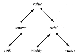
Figure 9.1
TwoWayType = RECORD
Parent :
 TwoWayNode
Value : {value type or pointer typeChild : ARRAY[1 . . 2] OF
 TwoWayNode
Visit : INTEGER
END
 . Visit is set to zero in each node when the traverse is complete. If the tree was initiated that way, TwoWayVisit leaves it unchanged. Clearly the Child field can be expanded to include more children.
procedure TwoWayVisit(twt) {O(n)p
 twt
twtwhile p
 NIL do
case of p
 .Visit
0 : PROCESS1(p)
p
 .Visit
  1
1q
 p
p  .Child[1]
if q
 NIL
NILthen p
 q
qendif
1 : PROCESS2(p)
p
 .Visit
  2
2q
 p
p  .Child[2]
if q
 NIL
NILthen p
 q
qendif
2 : PROCESS3(p)
p
 .Visit
  0
0p
 p
p  .Parent
endcase
endwhile
end {TwoWayVisitif p
 .Value = Wanted then return p endif
procedure xWayVisit(xwt) {O(n)p
 xwt
xwtwhile p

 NIL do
with p do
Visit
 (Visit + 1) MOD (x + 1)
PROCESS(Visit,p)
q
 Child[Visit]
if (q
 NIL) OR (Visit = 0)
then p
 q
qendif
endwith
endwhile
end {xWayVisit9.4 m-Way Search Trees
mWayNode = RECORD
Value : ARRAY[1 . . n] OF {value or pointer typeKey : ARRAY[1 . . n] OF {key typeptr : ARRAY[0 . . n] OF
 mWayNode
END {mWayNode
Figure 9.2
 i < n.
 i < n.
 i
i  n. (There is no Key[0].)
 i
i  n are m-way search trees.
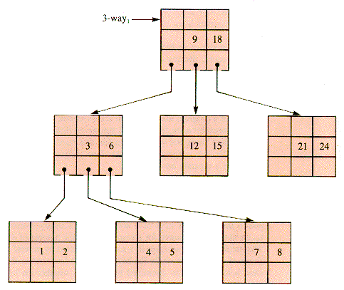
Figure 9.3
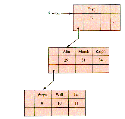
Figure 9.4
 mWayNode (a pointer to the parent of a node, Node) If this field is used, Node itself is sufficient to locate its parent node.
9.5 B-trees
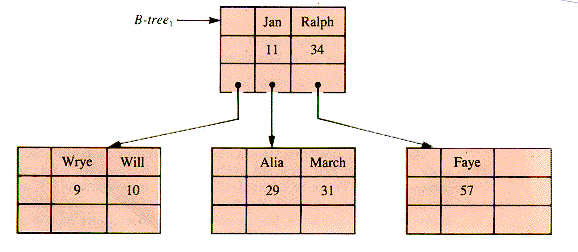
Figure 9.5

Figure 9.6
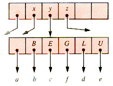
Figure 9.7
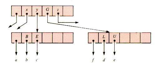
Figure 9.8
9.5.1 Creation and Splitting of B-tree Nodes
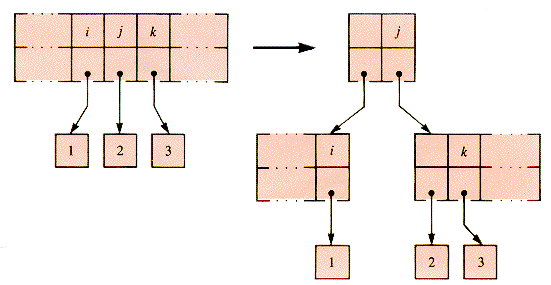
Figure 9.9
procedure Create(mwt,LefTree) {O(m)NEW(mwt)
with mwt do
ptr[[0]
 LefTree
Active
 0
0Up
 NIL
NILUpKey
 0
0for i = 1 to m do
ptr[i]
 NIL
NILnext i
endwith
end {Createprocedure NewKeyIn(Node,Ndex,NewKey,NewValue,SubTree) {O(m)with Node
 do
dok
 Ndex
Ndexfor i = Active downto k do
Value[i + 1]
 Value[i]
Key[i+1]
 Key[i]
ptr[i + 1]
 ptr[i]
if ptr [i]
 NIL
NILthen ptr[i]
 .UpKey
  ptr[i]
  .UpKey + 1
endif
next i
Value[k]
 NewValue
Key[k]
 NewKey
Active
 Active + 1
endwith
end {NewKeyInCreate(mwt,NIL)
NewKeyIn(mwt,1,NewKey,NewValue,NIL)
old
 mwt
mwtCreate(mwt, old)
NewKeyIn(mwt,1,NewKey,NewValue,SubTree)
procedure mWayScan(Node,ScanKey,Ndex,Found) {O(m)Found
 FALSE {ScanKey may be larger
Ndex
 Node
Node  .Active {than the keys in Node.
for i = 1 to Node
 .Active do
if ScanKey = Node
 .Key[i] {The search is complete.
then Ndex
 i
iFound
 TRUE
TRUEreturn
endif
if ScanKey < Node
 .Key[i] {The subtree to be searched
 {next has been located.then Ndex
 i - 1
i - 1exit
endif
next i
end {mWayScanprocedure mWaySearch(mwt,SearchKey,Node,Ndex,Found)
Node
 mwt
mwtParent
 mwt {O(m
  (mwt depth))
while Node
 NIL do
if Node
 .Active = m
then mWaySplit(Node,Ndex,NewKey,NewValue,SubTree)
NewKeyIn(Node,Ndex,NewKey,NewValue,SubTree)
endif
mWayScan(Node,SearchKey,Ndex,Found)
if Found then return endif {SearchKey is found in Node.Parent
 Node
NodeNode
 Node
Node  .ptr[Ndex]
endwhile
Node
 Parent {SearchKey is not in mwt.
end {mWaySearch .Key[q
 .UpKey], as shown in Figure 9.10.
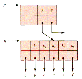
Figure 9.10
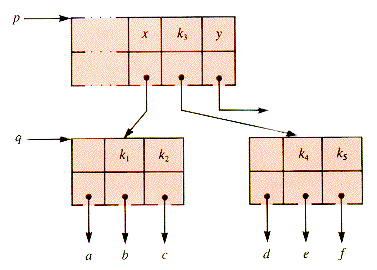
Figure 9.11
procedure mWaySplit(Node,Ndex,NewKey,NewValue,SubTree) {O(m)k
 INT(Node
  .Active/2 + 1) {The index of the key to
NEW(r) {be moved up one level.j
 1
1for i = k + 1 to Node
 .Active do {Shift the right
r
 .Value[j]
  Node
Node  .Value[i] {half of Node to r
r
 .Key[j]
  Node
Node .Kev[i]
r
 .ptr[j]
  Node
Node .ptr[i]
j
 j + 1
j + 1next i
r
 .ptr[0]
  Node
Node  .ptr[k]
j
 0
0for i = k to Node
 .Active do
if Node
 . ptr[i]
  NIL
NILthen Node
 .ptr[i]
  .Up
.Up  r
rNode
 .ptr[i]
  .UpKey
  j
jendif
j
 j + 1
j + 1next i
NewValue
 Node
Node  .Value[k]
NewKey
 Node
Node  . Key[k]
SubTree
 r
rNode
 .Active
  k - 1
k - 1r
 .Active
  m - k
m - kif Node
 .Up
.Up  NIL {Insert the middle key at the next
then Ndex
 Node
Node  .UpKey + 1 {higher level, at the right of
Node
 Node
Node  .Up {UpKey, locating the new node.
else Create(mwt,mwt) {A new node is needed. The oldNode
 .Up
.Up  mwt {mwt is the left child of the new.
Node
 .UpKey
  0
0Node
 mwt
mwtNdex
 1
1endif
r
 .Up
.Up  Node
Noder
 .UpKey
  Ndex
Ndexend {mWaySplit9.5.2 Insertion into a B-tree
procedure mWayIn(mwt,SearchKey,NewValue) {O(m  depth)
if mwt = NIL
then Create(mwt,NIL)
NewKeyIn(mwt,1,SearchKey,NewValue,NIL)
return
endif
mWaySearch(mwt,SearchKey,Node,Ndex,Found )
if Found {SearchKey is not really new.then return
else NewKeyIn(Node,Ndex +1,SearchKey,NewValue,NIL)
endif
end {mWayIn9.5.3 Deletion from a B-tree
function LeftMost(p) {O(depth)while p
 .ptr[0]
  NIL do
p
 p
p  .ptr[0]
endwhile
return p
end {LeftMostprocedure mWayOut(mwt, OutKey)
if mwt = NIL then return endif
mWaySearch(mwt,OutKey,Node,Ndex,Found)
if NOT Found then return endif {since OutKey is already goneSubTree
 Node
Node  .ptr[Ndex]
if SubTree
 NIL
NILthen SmallChild
 LeftMost(Subtree)
Node
 .Value[Ndex]
  SmallChild
  .Value[1]
Node
 .Key[Ndex]
  SmallChild
  .Key[1]
Node
 SmallChild
Ndex
 1
1endif
CutLeaf(Node,Ndex) {Now the key to be deleted is in a leaf node.end {mWayOutprocedure Compact(Node,Ndex) {O(m)with Node
 do
dofor i
 Ndex to Active - 1 do
Value[i]
 Valuel[i + 1]
Key[i]
 Key[i + 1]
if prt[i + 1]
 NIL
NILthen prt[i + 1]
 .UpKey
  1
1endif
ptr[Active]
 NIL
NILActive
 Active - 1
if Active = 0
then if ptr[0]
 NIL
NILthen Up
 .ptr[UpKey]
  ptr[0]
endif
if Up
 NIL
NILthen Up
 .ptr[UpKey]
  ptr[0]
else mwt
 ptr[0]
endif
DISPOSE(Node)
endif
endwith
end {Compact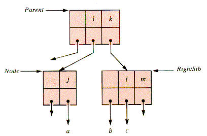
Figure 9.12
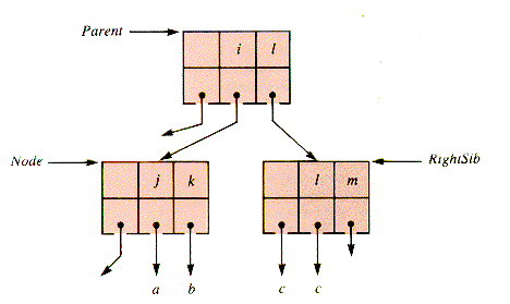
Figure 9.13
procedure ShiftLeft
p
 parent
NU
 Node
Node  .UpKey + 1
NA
 Node
Node  .Active + 1
RS
 RightSib
NewKeyIn(Node,NA,p
 .Key[NU],p
  .Value[NU],RS
  .ptr[0])
p
 .Value[NU]
  RS
RS  .Value[1]
p
 .Key[NU]
  RS
RS  .Key[1]
 RS
 .ptr[0]
  RS
RS  .ptr[1]
Compact(RS,1)
end {ShiftLeft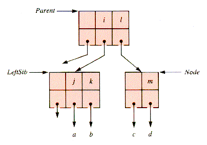
Figure 9.14
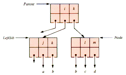
Figure 9.15
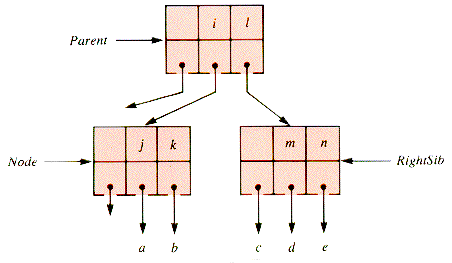
Figure 9.16
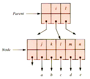
Figure 9.17
procedure ShiftDown(Node,RightSib) {O(m)p
 Parent
NU
 Node
Node  .UpKey + 1
NA
 Node
Node  .Active + 1
RS
 RightSib
NewKeyIn(Node,p
 .Key[NU],NA,p
  .Value[NU],RS
  .ptr[0])
for i = 1 to RS
 .Active do
NewKeyIn(Node,NA,RS
 .Key[i],RS
  .Value[i],RS
  .ptr[i])
next i
Ndex
 NU
NUNode
 Parent
DISPOSE(RS)
Compact(p,NU)
end {ShiftDownprocedure CutLeaf (Node,Ndex)
Limit
 INT((m + 1)/2 - 1) {O(m
  depth)
while Node
 mwt do
Compact(Node,Ndex) {Remove key from NodeSize
 Node
Node  .Active
if Size
 Limit then return endif {since no reshaping is required.
Parent
 Node
Node  .Up
.UpNU
 Node
Node  .UpKey + 1
RightSib
 Parent
  .ptr[NU]
LeftSib
 NIL
NILif NU > 1 then LeftSib
 Parent
  .ptr[NU - 2] endif
if RightSib
 NIL {Try to fill the hole at
 this level.
then if RightSib
 .Active > Limit
then ShiftLeft
return
endif
else if LeftSib
 .Active > Limit {LeftSib cannot be NIL.
then ShiftRight
return
endif
endif
if RightSib
 NIL {A key is moved down.
then ShiftDown(Node,RightSib)
else ShiftDown(LeftSib,Node)
endif
endwhile {The root node has been reached,Compact(Node,Ndex) {and a key shifted down from it.end {CutLeaf9.6 2-3-4 Trees (optional)

Figure 9.18
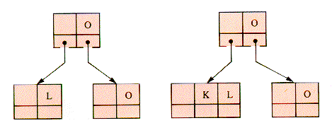
Figure 9.19
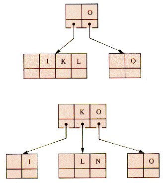
Figure 9.20
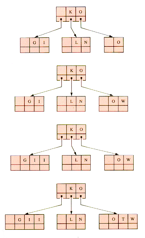
Figure 9.21

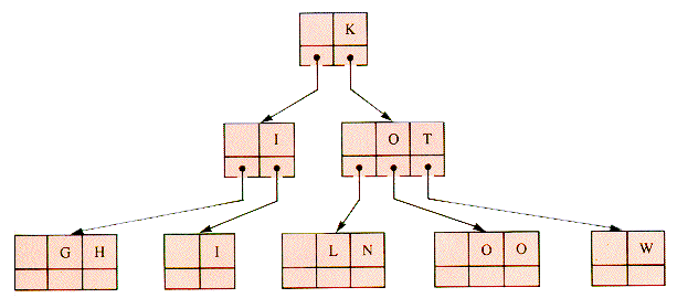
Figure 9.22
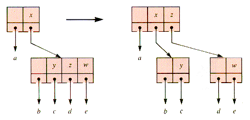
Figure 9.23
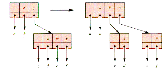
Figure 9.24
9.7 Sets and Their Trees (optional)
IF Token IN CodeSymbols THEN Accept (Token)
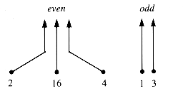
Figure 9.25
 .p is used for A[x]
  .p.
.p.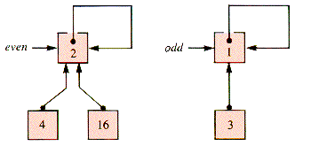
Figure 9.26
procedure NewSet(x) function QuickUnion(x,y) {0(1)x
 .p
.p  x x
x x  .p
.p  y
yend {NewSet return yend {QuickUnionfunction QuickFind(x) {O(depth)while x
 .p
.p  x do
x dox
 x
x  .p
.pendwhile
return x
end {QuickFind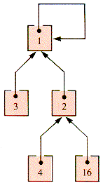
Figure 9.27
procedure CountUnion(x,y) {0(1)Total
 x
x  .c + y
  .c
.cif x
 .c > y
  .c
.cthen y
 .p
.p  x
xx
 .c
.c  Total
Totalelse x
 .p
.p  y
yy
 .c
.c  Total
Totalendif
end {CountUnion .p to Root.
function Find(x) {O(depth)Root
 x
xwhile Root
 .p
.p  Root do
Root
 Root
Root  .p
.pendwhile
while x
 Root do {collapsing
y
 x
x  .p
.px
 .p
.p  Root
Rootx
 y
yendwhile
return Root
end {Find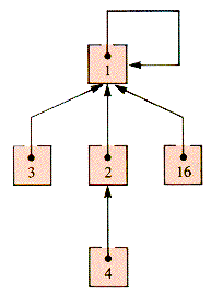
Figure 9.28
function HalFind(x) {O(depth)while x
 x
x  .p do
.p doy
 x
x  .p
.px
 .p
.p  y
y  .p
.px
 y
yendwhile
return x
end {HalFind .Rank > y
  .Rank, then x becomes the new root. If x
  .Rank = y
  .Rank, then y is the new root, and its rank is incremented (by one). The operation is:
function Union(x,y) {O(1)if x
 .Rank > y
  .Rank
.Rankthen y
 .p
.p  x
xreturn x
else if x
 .Rank = y
  .Rank
.Rankthen y
 .Rank
.Rank  y
y  .Rank + 1
endif
endif
x
 .p
.p  y
yreturn y
end {Union9.8 Trees as Decision Tools (optional)
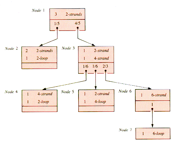
Figure 9.29
9.9 Game Trees (optional)
Summary
Exercises
Problems
Programs


