When a node to be deleted from a linearly linked list has been located, its removal requires a pointer to both of its immediate neighbors in the list--its predecessor as well as its successor. The same requirement makes some operations, such as the DeleteTail procedure of section 3.3.4, awkward. In an operation on a linear list where the predecessor of a node is required, the predecessor must be located with a search. One way to enhance access to neighboring nodes within a list is to weave two linked lists together to form a doubly linked list, as shown in Figure 6.1 :
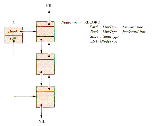
Figure 6.1
Procedures DeleteHead, InsertHead, and InsertTail are straightforward adaptations of single-linked list routines. With a simple return as a response to an empty list, DeleteTail is:
procedure DeleteTail(dList) {O(1)
if Empty then return endif
eTail
.Forth {NIL or u
UpTail
.Back
if Up = e
then Heade {singleton response
else Up.Forth
e
endif
DISPOSE(Tail)
TailUp
end {DeleteTailThe deletion of a node from the middle of such a list is relatively straightforward. To remove an already located p, the deletion procedure might follow the schema in Figure 6.2.
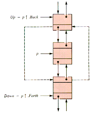
Figure 6.2
The relinking can be done with:
procedure UnDouble(dList,p) {O(1)
if Empty then return endif
Upp
.Back
Downp
.Forth
eTail
.Forth {NIL or u
if Down = e
then DeleteTail(dList)
return
endif
if Up = e
then DeleteHead(dList)
return
endif
Up.Forth
Down
Down.Back
Up
DISPOSE( p)
end {UnDoubleAn assumption made in UnDouble is a necessary condition for a list to be doubly linked; for any interior node (not Head or Tail):
p = p.Forth
.Back = p
.Back
.Forth
Program PG6.1 is appropriate at this point.
Double links are especially efficient in circular lists, such as that in Figure 6.3. There is no distinguishable position in such a list, although Q is the distinguished node. It can be convenient to let Q float from node to node in a sequence of "search and process" operations, pointing to the last (distinguished) node associated with an operation. Because such a ring has no natural head or tail, treating it as a stack or queue requires care.
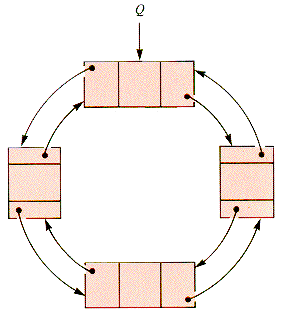
Figure 6.3
Exercises E6.1 and E6.2 are appropriate at this point.
6.2 n-braids
The doubly linked assumption can be relaxed for more general linked lists, as shown in Figure 6.4. The Forth list defines the sequence 1,2,3,4. The Back list defines the sequence 4,2,3,1. The independence of the Back and Forth linearly linked lists reintroduces the need to search for predecessors. The structure in Figure 6.4 is fundamentally two interwoven lists, a 2-braid, not a doubly linked list. A 2-braid can be used to simultaneously sequence one set of nodes in two ways. In general, an interweaving of n linear lists on one set of nodes (an n-braid) can be used to sequence the nodes in n ways without duplicating the nodes.
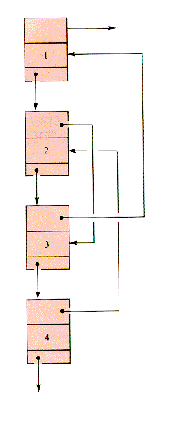
Figure 6.4
The nodes of an n-braid contain link fields associated with more than one list. Procedures to be applied to such nodes must either be written to process a specific braid or be generalized in some way. One way to generalize such procedures is to use an array of link-fields: Braid[1 . . n]. Then an index k is used to specify the braid link and hence to select braid k to be processed. It then requires very little alteration of standard list procedures to construct general braid procedures. In this chapter, we will assume that the following are available:
RingIn(b,p,q) inserts node p as the successor to node q into braid b, shown in Figure 6.5.
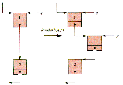
Figure 6.5
RingOut(b,q) deletes the successor of node q from braid b, shown in Figure 6.6.
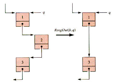
Figure 6.6
The search for q in both RingIn and RingOut may depend on the structure within which a braid lies and the starting point of the search.
Note: Insertion into and deletion from an n-braid involves location of the node in each braid. Disposal of a node must be delayed until it is deleted from all its braids.
Problem P6.1 is appropriate at this point.
6.3 Matrices and Graph Adjacency
The systems to which combinations of data structures can be applied are sometimes complex. Two models that are powerful simplifiers and organizers are commonly applied to such systems to make them accessible to analysis and design. These two models are the matrix and the graph. They are introduced very briefly here as necessary background for discussions in later parts of the book.
When the arithmetic operations ADDITION and MULTIPLICATION and their interactions are defined for tables, the tables become matrices. There is a strong analogy between the definition of such mathematical structures and computing structures such as ARRAY, STACK, and QUEUE. The operations of the structure MATRIX can even be defined algorithmically, in which case the mathematical structure and the data structure correspond very closely to each other.
The algorithmic definitions of the matrix operations ADDITION and MULTIPLICATION are:
For two n X m tables, A[1 . . n,1 . . m] and B[1 . . n, 1 . . m], added to form C[1 . . n,1 . . m], ADDITION is defined by:
For A[1 . . n, 1 . . p] and B [1 . . p, 1 . . m], multiplied to form the product C[1 . . n, 1 . . m], MULTIPLICATION is defined by:
Tables can be used to describe many systems, physical and conceptual. It is uncanny and satisfying that matrix operations often model the behavior of such systems. As an example, many systems can be modeled geometrically as a graph: informally, a collection of nodes joined by edges, as in Figure 6.7.
Graphs participated in the genesis of topology, may be involved in the demise of some management schemes, and certainly picture all networks, including those used to approximate topographies in models of agricultural regions.
Graphs depict the connections called edges between entities called vertices; that information may also be tabulated. The table associated with a graph is called its adjacency matrix. To tabulate a graph:
Number the nodes (as done in Figure 6.7) and associate both a row and a column of table G with each node.
If there is an edge connecting node i with node j, then G[i,j]
Figure 6.8 shows the graphs from Figure 6.7 in tabulated form.
One way to interpret these tables is that they select the pairs of nodes connected by a one-step path. A chain in a graph is a sequence of edges that lead from one node to another. Technically, if an edge is defined by the pair of nodes it connects, like {1,2} for the edge e in (a), then a chain is a sequence {N1,N2}, {N2,N3}, . . . , {Nn-1,Nn} that joins node N1 with node Nn. The charming effectiveness of mathematics appears when the graph tables are treated as matrices and raised to powers as Gc2 is in Figure 6.9.
An entry Gc2[i,j] is the number of chains of precisely two steps that joins Node i to Node j. Similarly, Gc3 tabulates the number of paths of length 3 that join pairs of nodes in the graph of example (c). Hence the powers of a graph matrix provide valuable information about the system modeled by the graph. This is not the only connection between matrices and graphs, but merely an illustration of the ubiquity of matrix operations.
Chapter 10 deals with graph representations as data structures. In this chapter, it is the mathematical nature of a matrix that determines the structure used to represent it; and that structure differs from those used in Chapter 10.
Exercise E6.3, problem P6.2, and program PG6.2 are appropriate at this point.
There is no need to restrict the linkage patterns of data elements to linear structures or even to combinations of linear structures. For example, four nodes may be linked as in Figure 6.10.
A simpler geometrical model for this pattern is a digraph (directed graph), which differs from a graph precisely because the edges possess direction, as shown in Figure 6.11.
Like a graph, a digraph model has an adjacency matrix, although a digraph matrix is not symmetric about the main diagonal (M[i,i], 1
Since edges in a digraph are directional, so are sequences that follow them from one vertex to another. The analog of a graph chain is a digraph path. It is still true that Mk[i,j] is the number of k-step paths from [i] to [j], as shown for this example in Figure 6.13.
Digraphs arise as models of such diverse systems as dominance relations in sociology and management, communication networks, and relations between data elements in the flight and ticket information of an airline. Data can be structured as a collection of nodes linked in the same pattern as the natural digraph model. Such a node structure is called a digraph list, also a general list.
Note: It is the digraph rather than the graph that corresponds most closely to data structures formed with pointers, because they are directional. In data structures that model graphs, two links represent each edge, one for each direction.
The design of fundamental operations like INSERT and DELETE become very application-dependent and sometimes difficult in a general list. A search through a digraph structure appears to be forbidding; nevertheless it is required in some applications. Hence there are algorithms for visiting each node of a general list, and a node may be processed in any desired way during the visit. One such algorithm is to be found in Part II, section M. A different visitation algorithm for general lists is the subject of section 7.7, where it serves as an example of a recursive algorithm. The traverse of a (restructured) general list can also be patterned very closely after the treatment of graphs in Chapter 10.
In many applications of graphs modeled by matrices and in other applications involving matrices, most of the entries are zero. Such a matrix is called a sparse matrix. A workable pair of definitions is that an N by N matrix is sparse if it contains O(N) nonzero entries and dense if it contains O(N2) nonzero entries.
The value of the nonzero entries in a sparse matrix as well as their location by row and column can be important, and a listing of the nonzero entries defines the zero entries by default if it is known to be complete. Any structure to which matrix operations are applied needs a row and column organization. It is nevertheless possible to trade simplicity and the independent access to a large and sparsely used storage space for complexity of structure coupled with more efficient use of storage. The trade of fast access for efficient storage is frequently made for problems that involve sparse matrices.
A number of data structures can be used to represent a sparse matrix:
1. SST (Sparse and Static Table). This structure is intrinsically static; not only is its storage allocation fixed, but it is also designed for a specific subset of the cells of the large (virtual) matrix it represents. It is excellent for some sparse table storage, as indicated in section 2.4, but difficult at best to adapt to the general situation of a changing (but still sparse) matrix.
2. MDC (Main Diagonal Circulation). The backbone of this structure is a collection of nodes, each representing a header for two circular lists: a row list and a column list. Each nonzero cell is represented by a node braided into one row list and one c
olumn list. This structure is detailed in Part II, section N.
3. AM (Adjacency Matrix) and AL (Adjacency List). These are the structures of choice tor supporting a graph traverse, and they are explored in Chapter 10.
4. HT (Hash Table). The indices of a cell in a large table can be used to form a hashed address in a smaller table. This approach depends on the discussions of hashing in Part II, sections B and L . It is the basis of PJ6. 1.
5. OL (Orthogonal Lists). A circular list of row headers and a circular list of column headers form the framework of row and column (circular) lists. Each cell in the array is braided into one row and one column list. This approach is discussed in section 6.5.
For all of these structures, the user is generally a procedure that accesses the matrix as a table, as would those of section 6.3 when applied to sparse matrices. The desired service is provided by STORE(i,j,x) and RETRIEVE(i,j).
Note: It may be possible to rewrite procedures that access a sparse matrix to make them "more efficient," but don't. The result tends to be logical spaghetti, which is hard to debug. Leave if for another course.
In all of these structures, deletion is awkward, and deletion can occur as the result of STORE. When an assignment is made to sparse matrix M, as done by M[i,j]
An existing node is to be updated:
A new node is to be inserted into M:
A node is to be deleted from M:
In the case of MDC and OL, deletion and insertion are made into both row and column braids with the RingIn and RingOut procedures of section 6.2.
An example of a very small but relatively sparse matrix is:
This matrix may be represented by an interwoven collection of circular lists in which there are (2n+1) header nodes and precisely as many cell nodes as needed for nonzero entries. Every node is braided into a row braid and a column braid, and the headers are distinguished by having either a row or a column index that is illegal, as in Figure 6.14, where 0 is the illegal index.
Exercise E6.4 is appropriate at this point.
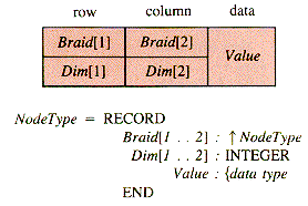
General procedures such as RingIn and RingOut (section 6.2) are applicable to the OL structure if node records use indexed braid pointers and dimension identifiers (for row and column):
Both STORE and RETRIEVE involve finding the correct header, then the predecessor of the node to be accessed. Header location for row or column dex is an adaptation of LT (section 3.3.2):
The appropriate row and column can then be located by:
A very similar routine locates the predecessor of the node with a given index in the other direction, within a given braid:
With these tools available, RETRIEVE is straightforward: the node in the position where M[i,j] is expected is located as p. If M[i,j] is not present, p
STORE is more complex, since it may involve inserting or deleting a node. One version, tuned for clarity but not for efficiency, is:
Program PG6.3 is appropriate at this point.
At the lowest level, the main store of a computing system is a large array, part of it preempted by housekeeping procedures necessary for interface of the system to the outside world and to working programs. The operating system, called on by compiler-generated instructions, is asked to provide storage on demand from the main store each time a program is activated and each time a utility routine such as NEW is executed.
The main store array has a maximum address, like other arrays. If memory is partitioned among several users, each user has a segment available which--to that user--appears to be the entire store. No other user has access to this segment of memory at the same time.
If memory is shared, then its management becomes delicate, because a user may change values in memory cells accessed by other users. Memory is not actually increased in size by sharing, even though its utilization may be greater during a given span of time it would be for unshared memory. The issues involved with shared memory are dealt with in the study of operating systems.
In this section we assume that a single user--while active--has command of a store of fixed size. With that assumption, a program that manages a block of memory by allocating subblocks of fixed size behaves like the memory-management process of an operating system.
Consider a time-sharing system that has a finite number of active programs resident in memory, each waiting for or using a slice of processor time. A program is allocated storage space when it is activated. The amount to be allocated is specified when it is compiled, and no more space becomes available during execution. An apparent limitation of this scheme is that dynamic allocation of memory for pointer variables is not allowed. In some implementations the space allotted to a program may be large enough to allow some dynamic allocation during execution, but the allocation cannot exceed a set maximum.
A request for the allocation of memory for a new program comes from a scheduling process, the scheduler, to the memory management program, Mem. If memory is available, it is provided by Mem, and the program is activated. From time to time, a program completes its execution and becomes passive. When this happens Mem is informed and the storage occupied by the formerly active program is released; it is free and may be used for activation of new programs.
Note: The mangement scheme presented here is a model, based on data structures that have been described in previous sections. More sophisticated structures are applied in practice.
In practice, memory is soon broken into segments occupied by active programs, separated by segments of free storage. The blocks of free storage are linked together by Mem in a circular list called Avail, like the one in Figure 6.15. The release of each of the active blocks 1,3,5,6, and 7 differs somewhat from the release of the others.
The guiding principle for release is that when a block is freed, it is to be joined with any contiguous free blocks, enlarging them. The newly freed block is not to be joined to free blocks separated from it by active programs. This is one of several possible strategies, one that allows "quick release."
The catch to this strategy is that "contiguous" means adjoining, in absolute location, to blocks that are not on the Avail list. Blocks are adjoining on the availability list because of the sequence of entries into and exits from Avail, not because of their absolute location.
The property of being contiguous is bidirectional in memory, and so a natural way to link together all blocks, free and active, is as a doubly linked list, Store, illustrated in Figure 6.16. Mem is exogenous; it uses nodes that are records that point to memory blocks, although an operating system could store the linkage and other information in the blocks themselves (because it has the use of machine instructions that access any cell in any available way).
If block 3 is deactivated, then blocks 2,3, and 4 are collapsed into one block, say block 2, and the resulting structure is depicted in Figure 6.17.
The information required in a block node is an identifier (for active programs, three pointers (two for Store and one for Avail), the absolute starting address, and the size of the block:
The two major operations are the release of active blocks and the activation of a program. Both are nontrivial.
Both doubly linked lists and circular lists were used without introducing much complexity in previous chapters, and so it might seem that their action in concert would not be complicated. In fact, combined structures can present a much more complex management task.
6.6.1 The Release of an Active Block (optional)
6.6.2 The Activation of a Program (optional)
Given a node p that is to be deactivated, several possibilities must be distinguished in the procedure UnLeash that frees it. With the use of
the possibilities are delineated in Table 6.1. A straightforward implementation of this organization will produce a nest of if . . . then . . . else constructs. An alternative way to orchestrate the release operation is to define simpler subtasks and then structure the way they work together to solve the overall task.
If Up is free, then p and Up may be joined to form a single free block. From the perspective of Up, it is simply extended to engulf p. Hence, a natural operation is the joining of a lower block to an upper block, say Join(dList,q), where q points to the upper block in a doubly linked list, dList. Then Join(dList,Up) can be followed by deletion of the lower block from dList with a standard DELETE operation, UnDouble(dlist,p). (In this example, the specific list involved will be called Store.) If p is not absorbed by Up it is inserted into Avail with Free( p). If Up engulfs p the combined block is renamed p.
If Down is free, then p and Down may be joined; their joining can be considered an engulfment of p by Down. When p and Down are combined with Bind(Down) block p must be deleted from Avail as well as from Store. This deletion from Avail is simply a DELETE operation of a node from a circular list.
When the special cases are taken care of, UnLeash becomes:
The details of Join, Free, and Bind are left to the problems.
Problems P6.3 and P6.4 are appropriate at this point.
When a request (by one part of the operating system to the activation routine) is made to activate a program of size s, several possibilities must be distinguished:
1. There is a block p in Avail for which p
2. There are blocks in Avail with size at least as large as s (but not necessarily an exact fit).
3. There is no single block in Avail large enough to contain the program, but if active programs are shifted in absolute location, several blocks in Avail can be joined to form a block larger than s.
4. The total of the sizes of the blocks in Avail is less than s, and so the request cannot be granted at all.
The shifting-and-collapsing operation implied in possibility 3 is called garbage collection. It is not always clear just when garbage collection should be done and how. Automatic garbage collection can be incorporated into the release operation so that, on release, all programs are shifted: only one free block ever exists. Analysis reveals that this is a wasteful overhead in most systems. The assumption here is that it is to be done if no single block is of size s or greater, but the sum of all free sizes is greater than s.
Possibility 2 includes possibility 1; several strategies have been devised to deal with it, and there are various implementations of them. In general, some piece of the free block is left over when there is no exact fit. A large number of activation-deactivation cycles can leave many blocks on the Avail list too small to be useful for active programs. One way to alleviate this problem is to allocate an entire block if it is a "close fit." The effectiveness of this technique is naturally dependent on the statistics of an application. Strategies for allocating blocks as large as s to a program include:
first-fit: Work around Avail until a free block is located as p, for which p
best-fit: Search all of Avail, and return p, where (p
worst-fit: Search all of Avail, and return p, where p
Allocation for any of these strategies involves transferring the program to p and unlinking p from Avail. They are not particularly difficult to program, and they are left to the problems.
It is convenient to move an active program into the bottom of a free block so that, if the excess forms a free block, it is already linked into Avail, although its size has changed.
The ideas of first-fit, best-fit, and worst-fit are used as strategies for solving other problems (such as bin-packing, the solution to which is related to the solution of a huge collection of important problems).
Problems P6.5-P6.7 are appropriate at this point.
Garbage collection in practice involves difficulties outside the scope of this book. For one thing, programs are moved, and they must execute after being moved. If the active blocks are treated as though they can be moved simply by updating the fields of their records, then garbage collection is a relatively straight-forward shifting operation. It is convenient to shift active blocks upward in memory, leaving a single free block at the bottom of storage. Hence Avail can be ignored during the shift and then reinitialized as a single node.
Writing a simulation of memory management that explores the effect of activation strategies and the effect of the distributions of program size and execution times is a substantial project as a class assignment. It is, however, a minor task compared to writing an operating system.
Projects PJ6.1-PJ6.3 are appropriate at this point.
Control traffic flows over links in one direction only, and so it is sometimes useful to trade space for the convenience of multiple-link paths. The most straightforward multiple-path structure is the doubly linked list, but lists may be interwoven in almost any pattern to form n-braids. Deletion and insertion in interwoven lists requires more care than in singly linked lists; the doubly linked list is intermediate in this respect.
The adjacency matrix, the graph, and the digraph are models with great power to simplify, synthesize, and organize. All three correspond to data structures of wide application and provide background for understanding them.
Matrices (and other tables) commonly waste space because many cells contain a standard value (such as zero). A number of structures are available for dealing with this situation and are treated in section 2.7; Part II, sections B, L, and N; section 6.4; Chapter 10; and PJ6.1. The Orthogonal List structure is detailed in section 6.4. This structure and the one detailed in Part II, section N, represent cells of the matrix as nodes braided into circular lists.
One (simplified) model of the dynamic allocation of memory in a computing system is a doubly linked list of blocks that contain either active programs or available storage. The available storage blocks are also on an interwoven circular list. Activating and deactivating programs presents a number of interesting problems not restricted to management of the structures themselves.
Exercises immediate applications of the text material
E6.1 Write an insertion procedure for a doubly linked list, as discussed in section 6.1.
E6.2 Write the procedures for both insertion and deletion in a doubly linked circular list.
E6.3 Determine the number of two-step and the number of three-step paths for graphs (a) and (b) of section 6.3, and verify by calculating the products Ga2, Ga3, Gb2, and Gb3.
E6.4 Draw the graphs (a) and (b) of section 6.3 as sparse matrix lists.
Problems not immediate, but requiring no major extensions of the text material
P6.1 Write procedures Ringln and RingOut of section 6.2 for nodes in an n-braid.
P6.2 Deterrnine the timing functions of AddMatrix and MultiMatrix of section 6.3.
P6.3 Write the procedure Join of section 6.6.1.
P6.4 Write the procedure UnDouble of section 6.6.1.
P6.5 Write a first-fit strategy procedure Firstfit for locating storage in Avail as described in section 6.6.2. Return NIL if no free block is large enough.
P6.6 Write a best-fit strategy procedure Bestfit for locating storage in Avail as described in section 6.6.2. Return NIL if no free block is large enough.
P6.7 Write a worst-fit strategy procedure WorstFit for locating storage in Avail as described in section 6.6.2. Return NIL if no free block is large enough.
Programs for trying it yourself
PG6.1 Write a program that inputs a sequence of paired names and test scores and puts them together in a two-link record. The records are to be linked so that they are in order alphabetically by one sequence of links, and in order by score in another sequence of links. Display the records in alphabetic order, on a line with their score successor, and then vice versa.
PG6.2 Write a program that will accept a sequence of edges (pairs of nodes), and calculate the number of k-fold paths from node i to node j for any specified i, j, and k.
PG6.3 Write a program designed around an entry loop that allows a user to insert and retrieve values from an n x n Orthogonal List form of a sparse matrix (as described in section 6.5).
Projects for fun; for serious students
PJ6.1 (Assumes knowledge of Part II, sections B and L.) Investigate the hashing of a table T[1 . . 30,1 . . 30] into HT[1 . . 10,1 . . 10] . The values in T are all to be either 0 or 1. Start with a loading of HT of 20 percent and determine the mean number of collisions generated by random retrievals and by random assignments, half of which are zero. Determine the loading after 20, 40, . . ., 100 assignments. Repeat this experiment for greater initial loading of HT.
PJ6.2 Write an emulation of memory management as described in section 6.6. The user should be able to activate or deactivate programs by name on command.
PJ6.3 Write a simulation of memory management as described in section 6.6. The user should be able to specify several control parameters and the mean and standard deviations for program sizes. Control parameters should include the number of activations and deletions, fitting strategy, and the "closeness" factor.
function AddMatrix(A,B) {O(n2)for i = 1 to n
for j = 1 to m
C[i,j]
 A[i,j] + B[i,j]
next j
next i
return C
end {AddMatrixfunction MultiMatrix(A,B) {O(n3)for i = 1 to n
for j = 1 to m {C[i,j] =  A[i,p] X B[p,j]
Sum
 0
0for k = 1 to p
Sum
 Sum + A[i,k] * B[k,j]
next k
C[i,j]
 Sum
Sumnext j
next i
return C
end {MultiMatrix
Figure 6.7
 1, otherwise G[i,j]
  0.
0.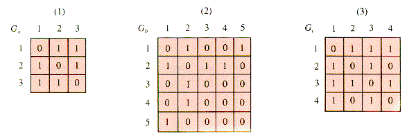
Figure 6.8
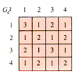
Figure 6.9
6.3.1 Directed Graphs
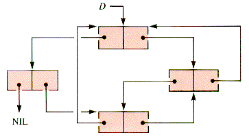
Figure 6.10
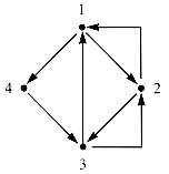
Figure 6.11
 i
i Max) in contrast to the adjacency matrix of a graph. An entry of 1 in M[i,j] for a digraph signifies a directed arc (an edge) from node i to node j. An edge is thus an ordered pair, (i,j). For the example above, the adjacency matrix M is shown in Figure 6.12.
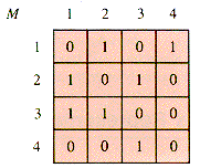
Figure 6.12
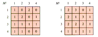
Figure 6.13
6.4 Sparse Matrix Representation
 x, several possibilities must be distinguished:
M[i,j]
 0 and x
  0
0M[i,j]
 0 and x
  0
0M[i,j]
 0 and x = 0
6.5 The Orthogonal List (optional)
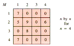
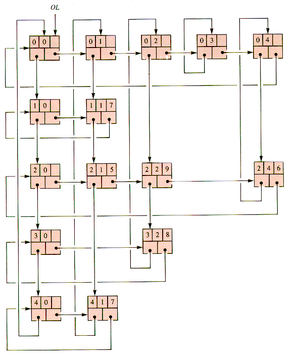
Figure 6.14
function FindBraid(Other,dex) {0(n)b
 (Other MOD 2) + 1
Head
 OL
OL  .Braid[Other]
while Head
 OL do
OL doif Head
 .Dim[b] = dex
then exit endif
Head
 Head
Head  .Braid[Other]
endwhile
return Head
end {FindBraidRow
 FindBraid(2,i)
Col
 FindBraid(1,j)
function FindPred(Head,b,dex) {O(n)Pred
 Head
Heads
 Head
Head  .Braid[b]
Other
 (b MOD 2) + 1
while s
 Head do
if s
 .Dim[Other]
  dex
dexthen exit endif
Pred
 s
ss
 s
s  .Braid[b]
endwhile
return Pred
end {FindPred .Braid[1] will not have the correct column index:
function Retrieve(i,j) {O(n)Row
 FindBraid(2,i)
RowPred
 FindPred(Row,1,j)
p
 RowPred
  .Braid[1]
if p
 .Dim[2]
  j
jthen return 0
else return p
 .Value
endif
end {Retrieveprocedure Store(i,j,x) {O(n)Row
 FindBraid(2,i)
Col
 FindBraid(1,j)
RowPred
 FindPred(Row,1,j)
ColPred
 FindPred(Col,2,i)
p
 RowPred
  .Braid[1]
if x = 0
then if p
 .Dim[2] = j {M[i,j] is in the matrix
then RingOut(1,RowPred)
RingOut(2,ColPred)
DlSPOSE(p)
endif
else if p
 .Dim[2] = j {M[i,j] is in the matrix
then p
 .Value
  x
xelse NEW(n)
n
 .Value
  x
xn
 .Dim[1]
  i
in
 .Dim[2]
  j
jRingIn(1,RowPred,n)
RingIn(2,ColPred,n)
endif
endif
end {Store6.6 A Dynamic Storage Allocation Model (optional)
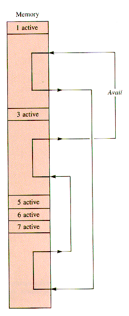
Figure 6.15
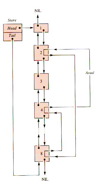
Figure 6.16
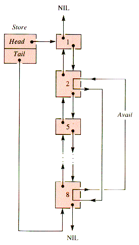
Figure 6.17
BlockType = RECORD
id : ARRAY[1 .. 20] OF CHAR
Back :
 BlockType {Store
Forth :
 BlockType {Store
Next :
 BlockType {Avail
Start : INTEGER
Size : INTEGER
END {BlockType6.6.1 The Release of an Active Block (optional)
Up
 p
p  .Back
.BackDown
 p
p  .Forth
Table 6.1
Up = NIL Down = NIL Avail was empty and now is to contain a single node, p.
Down
 NIL Down
  .next = NIL Down is active; it
 cannot be joined to p,
and so p is added as a
new node to Avail.
Down
 .Next
.Next  NIL Down is free; it is
 already in Avail, and so
it can be updated to engulf p.
Up
 NIL Down = NIL Up
  .Next = NIL Up is active; it cannot be
 joined to p, and so p is
added as a new node to Avail.
Up
 .Next
.Next  NIL Up is free; it is already
 in Avail, and so it can be
updated to engulf p.
Down
 NIL Up
  .Next = NIL Up is active; it cannot be
 joined to p. However, Down
may be either free or active,
and two cases result.
Up
 .Next
.Next  NIL Up is free; it is already
 in Avail, and so it can be
updated to engulf p.
However, Down may be either
free or active, and two cases
result.
procedure UnLeash(p)
Up
 p
p  .Back
.BackDown
 p
p  .Forth
if Up
 NIL
NILthen if Up
 .Next
.Next  NIL
NILthen Join(Store,p) {join p to UpUnDouble(Store,p)
p
 Up
Upelse Free(p)
endif
else Free(p)
endif
if Down
 NIL
NILthen if Down
 .Next
.Next  NIL {join (new) p to Down
then Bind(Down)
UnDouble(Store,p)
endif
endif
end {UnLeash6.6.2 The Activation of a Program (optional)
 .Size = s.
 .Size
.Size  s, and then return p.
 .Size - s)
  0 is minimal.
 .Size - s is maximal and at least 0.
Summary
Exercises
Problems
Programs
Projects


