Next Chapter Return to Table of Contents Previous Chapter

CHAPTER 13: BINARY SEARCH TREES

Search trees are data structures that support many dynamic-set operations, including SEARCH, MINIMUM, MAXIMUM, PREDECESSOR, SUCCESSOR, INSERT, and DELETE. Thus, a search tree can be used both as a dictionary and as a priority queue.

Basic operations on a binary search tree take time proportional to the height of the tree. For a complete binary tree with n nodes, such operations run in (lg n) worst-case time. If the tree is a linear chain of n nodes, however, the same operations take (n) worst-case time. We shall see in Section 13.4 that the height of a randomly built binary search tree is O(lg n), so that basic dynamic-set operations take (lg n) time.

In practice, we can't always guarantee that binary search trees are built randomly, but there are variations of binary search trees whose worst-case performance on basic operations can be guaranteed to be good. Chapter 14 presents one such variation, red-black trees, which have height O(lg n). Chapter 19 introduces B-trees, which are particularly good for maintaining data bases on random-access, secondary (disk) storage.

After presenting the basic properties of binary search trees, the following sections show how to walk a binary search tree to print its values in sorted order, how to search for a value in a binary search tree, how to find the minimum or maximum element, how to find the predecessor or successor of an element, and how to insert into or delete from a binary search tree. The basic mathematical properties of trees were introduced in Chapter 5.

13.1 What is a binary search tree?

A binary search tree is organized, as the name suggests, in a binary tree, as shown in Figure 13.1. Such a tree can be represented by a linked data structure in which each node is an object. In addition to a key field, each node contains fields left, right, and p that point to the nodes corresponding to its left child, its right child, and its parent, respectively. If a child or the parent is missing, the appropriate field contains the value NIL. The root node is the only node in the tree whose parent field is NIL.

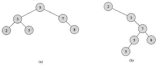
Figure 13.1 Binary search trees. For any node x, the keys in the left subtree of x are at most key[x], and the keys in the right subtree of x are at least key[x]. Different binary search trees can represent the same set of values. The worst-case running time for most search-tree operations is proportional to the height of the tree. (a) A binary search tree on 6 nodes with height 2. (b) A less efficient binary search tree with height 4 that contains the same keys.

The keys in a binary search tree are always stored in such a way as to satisfy the binary-search-tree property:

Let x be a node in a binary search tree. If y is a node in the left subtree of x, then key[y] key[x]. If y is a node in the right subtree of x, then key[x] key[y].

Thus, in Figure 13.1(a), the key of the root is 5, the keys 2, 3, and 5 in its left subtree are no larger than 5, and the keys 7 and 8 in its right subtree are no smaller than 5. The same property holds for every node in the tree. For example, the key 3 in Figure 13.1(a) is no smaller than the key 2 in its left subtree and no larger than the key 5 in its right subtree.

The binary-search-tree property allows us to print out all the keys in a binary search tree in sorted order by a simple recursive algorithm, called an inorder tree walk. This algorithm derives its name from the fact that the key of the root of a subtree is printed between the values in its left subtree and those in its right subtree. (Similarly, a preorder tree walk prints the root before the values in either subtree, and a postorder tree walk prints the root after the values in its subtrees.) To use the following procedure to print all the elements in a binary search tree T, we call INORDER-TREE-WALK( root[T]).

INORDER-TREE-WALK(x)

1  if x  NIL

2      then INORDER-TREE-WALK (left[x])

3           print key[x]

4           INORDER-TREE-WALK (right[x])

As an example, the inorder tree walk prints the keys in each of the two binary search trees from Figure 13.1 in the order 2, 3, 5, 5, 7, 8. The correctness of the algorithm follows by induction directly from the binary-search-tree property. It takes (n) time to walk an n-node binary search tree, since after the initial call, the procedure is called recursively exactly twice for each node in the tree--once for its left child and once for its right child.

Exercises

13.1-1

Draw binary search trees of height 2, 3, 4, 5, and 6 on the set of keys {1, 4, 5, 10, 16, 17, 21}.

13.1-2

What is the difference between the binary-search-tree property and the heap property (7.1)? Can the heap property be used to print out the keys of an n-node tree in sorted order in O(n) time? Explain how or why not.

13.1-3

Give a nonrecursive algorithm that performs an inorder tree walk. (Hint: There is an easy solution that uses a stack as an auxiliary data structure and a more complicated but elegant solution that uses no stack but assumes that two pointers can be tested for equality.)

13.1-4

Give recursive algorithms that perform preorder and postorder tree walks in (n) time on a tree of n nodes.

13.1-5

Argue that since sorting n elements takes (n lg n) time in the worst case in the comparison model, any comparison-based algorithm for constructing a binary search tree from an arbitrary list of n elements takes (n lg n) time in the worst case.

13.2 Querying a binary search tree

The most common operation performed on a binary search tree is searching for a key stored in the tree. Besides the SEARCH operation, binary search trees can support such queries as MINIMUM, MAXIMUM, SUCCESSOR, and PREDECESSOR. In this section, we shall examine these operations and show that each can be supported in time O(h) on a binary search tree of height h.

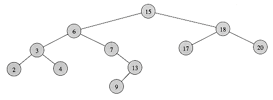
Figure 13.2 Queries on a binary search tree. To search for the key 13 in the tree, the path 15 6 7 13 is followed from the root. The minimum key in the tree is 2, which can be found by following left pointers from the root. The maximum key 20 is found by following right pointers from the root. The successor of the node with key 15 is the node with key 17, since it is the minimum key in the right subtree of 15. The node with key 13 has no right subtree, and thus its successor is its lowest ancestor whose left child is also an ancestor. In this case, the node with key 15 is its successor.

Searching

We use the following procedure to search for a node with a given key in a binary search tree. Given a pointer to the root of the tree and a key k, TREE-SEARCH returns a pointer to a node with key k if one exists; otherwise, it returns NIL.

TREE-SEARCH (x, k)

1 if x = NIL or k = key[x]

2     then return x

3  if k < key[x]

4     then return TREE-SEARCH (left[x], k)

5     else return TREE-SEARCH (right[x], k)

The procedure begins its search at the root and traces a path downward in the tree, as shown in Figure 13.2. For each node x it encounters, it compares the key k with key[x]. If the two keys are equal, the search terminates. If k is smaller than key[x], the search continues in the left subtree of x, since the binary-search-tree property implies that k could not be stored in the right subtree. Symmetrically, if k is larger than key[k], the search continues in the right subtree. The nodes encountered during the recursion form a path downward from the root of the tree, and thus the running time of TREE-SEARCH is O(h), where h is the height of the tree.

The same procedure can be written iteratively by "unrolling" the recursion into a while loop. On most computers, this version is more efficient.

ITERATIVE-TREE-SEARCH (x,k)

1  while x  NIL and k  key[x]

2      do if k < key[x]

3            then x  left[x]

4            else x  right[x]

5  return x

Minimum and maximum

An element in a binary search tree whose key is a minimum can always be found by following left child pointers from the root until a NIL is encountered, as shown in Figure 13.2. The following procedure returns a pointer to the minimum element in the subtree rooted at a given node x.

TREE-MINIMUM (x)

1  while left[x]  NIL

2      do x  left[x]

3  return x

The binary-search-tree property guarantees that TREE-MINIMUM is correct. If a node x has no left subtree, then since every key in the right subtree of x is at least as large as key[x], the minimum key in the subtree rooted at x is key[x]. If node x has a left subtree, then since no key in the right subtree is smaller than key[x] and every key in the left subtree is not larger than key[x], the minimum key in the subtree rooted at x can be found in the subtree rooted at left[x].

The pseudocode for TREE-MAXIMUM is symmetric.

TREE-MAXIMUM (x)

1  while right[x]  NIL

2      do x  right[x]

3  return x

Both of these procedures run in O(h) time on a tree of height h, since they trace paths downward in the tree.

Successor and predecessor

Given a node in a binary search tree, it is sometimes important to be able to find its successor in the sorted order determined by an inorder tree walk. If all keys are distinct, the successor of a node x is the node with the smallest key greater than key[x]. The structure of a binary search tree allows us to determine the successor of a node without ever comparing keys. The following procedure returns the successor of a node x in a binary search tree if it exists, and NIL if x has the largest key in the tree.

TREE SUCCESSOR(x)

1  if right[x]  NIL

2      then return TREE-MINIMUM(right[x])

3  y  p[x]

4  while y  NIL and x = right[y]

5       do x  y

6          y  p[y]

7  return y

The code for TREE-SUCCESSOR is broken into two cases. If the right subtree of node x is nonempty, then the successor of x is just the left-most node in the right subtree, which is found in line 2 by calling TREE-MINIMUM(right[x]). For example, the successor of the node with key 15 in Figure 13.2 is the node with key 17.

On the other hand, if the right subtree of node x is empty and x has a successor y, then y is the lowest ancestor of x whose left child is also an ancestor of x. In Figure 13.2, the successor of the node with key 13 is the node with key 15. To find y, we simply go up the tree from x until we encounter a node that is the left child of its parent; this is accomplished by lines 3-7 of TREE-SUCCESSOR.

The running time of TREE-SUCCESSOR on a tree of height his O(h), since we either follow a path up the tree or follow a path down the tree. The procedure TREE-PREDECESSOR, which is symmetric to TREE-SUCCESSOR, also runs in time O(h).

In summary, we have proved the following theorem.

Theorem 13.1

The dynamic-set operations SEARCH, MINIMUM, MAXIMUM, SUCCESSOR, and PREDECESSOR can be made to run in O(h) time on a binary search tree of height h.

Exercises

13.2-1

Suppose that we have numbers between 1 and 1000 in a binary search tree and want to search for the number 363. Which of the following sequences could not be the sequence of nodes examined?

a. 2, 252, 401, 398, 330, 344, 397, 363.

b. 924, 220, 911, 244, 898, 258, 362, 363.

c. 925, 202, 911, 240, 912, 245, 363.

d. 2, 399, 387, 219, 266, 382, 381, 278, 363.

e. 935, 278, 347, 621, 299, 392, 358, 363.

13.2-2

Professor Bunyan thinks he has discovered a remarkable property of binary search trees. Suppose that the search for key k in a binary search tree ends up in a leaf. Consider three sets: A, the keys to the left of the search path; B, the keys on the search path; and C, the keys to the right of the search path. Professor Bunyan claims that any three keys a A, b B, and c C must satisfy a b c. Give a smallest possible counterexample to the professor's claim.

13.2-3

Use the binary-search-tree property to prove rigorously that the code for TREE-SUCCESSOR is correct.

13.2-4

An inorder tree walk of an n-node binary search tree can be implemented by finding the minimum element in the tree with TREE-MINIMUM and then making n - 1 calls to TREE-SUCCESSOR. Prove that this algorithm runs in (n) time.

13.2-5

Prove that no matter what node we start at in a height-h binary search tree, k successive calls to TREE-SUCCESSOR take O(k + h) time.

13.2-6

Let T be a binary search tree, let x be a leaf node, and let y be its parent. Show that key[y] is either the smallest key in T larger than key[x] or the largest key in the tree smaller than key[x].

13.3 Insertion and deletion

The operations of insertion and deletion cause the dynamic set represented by a binary search tree to change. The data structure must be modified to reflect this change, but in such a way that the binary-search-tree property continues to hold. As we shall see, modifying the tree to insert a new element is relatively straightforward, but handling deletion is somewhat more intricate.

Insertion

To insert a new value v into a binary search tree T, we use the procedure TREE-INSERT. The procedure is passed a node z for which key[z] = v, left[z] = NIL, and right[z] = NIL. It modifies T and some of the fields of z in such a way that z is inserted into an appropriate position in the tree.

TREE-INSERT(T,z)

1  y  NIL

2  x  root[T]

3  while x  NIL

4       do y  x

5          if key[z] < key[x]

6             then x  left[x]

7             else x  right[x]

8  p[z]  y

9  if y = NIL

10      then root[T]  z

11      else if key[z] < key[y]

12              then left[y]  z

13              else right[y]  z

Figure 13.3 shows how TREE-INSERT works. Like the procedures TREE-SEARCH and ITERATIVE-TREE-SEARCH, TREE-INSERT begins at the root of the tree and traces a path downward. The pointer x traces the path, and the pointer y is maintained as the parent of x. After initialization, the while loop in lines 3-7 causes these two pointers to move down the tree, going left or right depending on the comparison of key[z] with key[x], until x is set to NIL. This NIL occupies the position where we wish to place the input item z. Lines 8-13 set the pointers that cause z to be inserted.

Like the other primitive operations on search trees, the procedure TREE-INSERT runs in O(h) time on a tree of height h.

Deletion

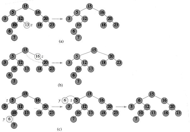
The procedure for deleting a given node z from a binary search tree takes as an argument a pointer to z. The procedure considers the three cases shown in Figure 13.4. If z has no children, we modify its parent p[z] to replace z with NIL as its child. If the node has only a single child, we "splice out" z by making a new link between its child and its parent. Finally, if the node has two children, we splice out z's successor y, which has no left child (see Exercise 13.3-4) and replace the contents of z with the contents of y.

The code for TREE-DELETE organizes these three cases a little differently.

Figure 13.3 Inserting an item with key 13 into a binary search tree. Lightly shaded nodes indicate the path from the root down to the position where the item is inserted. The dashed line indicates the link in the tree that is added to insert the item.

Figure 13.4 Deleting a node z from a binary search tree. In each case, the node actually removed is lightly shaded. (a) If z has no children, we just remove it. (b) If z has only one child, we splice out z. (c) If z has two children, we splice out its successor y, which has at most one child, and then replace the contents of z with the contents of y.

TREE-DELETE(T, z)

1  if left[z] = NIL or right[z] = NIL

2      then y  z

3      else y  TREE-SUCCESSOR(z)

4  if left[y]  NIL

5      then x  left[y]

6      else x  right[y]

7  if x  NIL

8      then p[x]  p[y]

9  if p[y] = NIL

10      then root[T]  x

11      else if y = left[p[y]]

12              then left[p[y]]  x

13              else right[p[y]]  x

14  if y  z

15      then key[z]  key[y]

16            If y has other fields, copy them, too.

17  return y

In lines 1-3, the algorithm determines a node y to splice out. The node y is either the input node z (if z has at most 1 child) or the successor of z (if z has two children). Then, in lines 4-6, x is set to the non-NIL child of y, or to NIL if y has no children. The node y is spliced out in lines 7-13 by modifying pointers in p[y] and x. Splicing out y is somewhat complicated by the need for proper handling of the boundary conditions, which occur when x = NIL or when y is the root. Finally, in lines 14-16, if the successor of z was the node spliced out, the contents of z are moved from y to z, overwriting the previous contents. The node y is returned in line 17 so that the calling procedure can recycle it via the free list. The procedure runs in O(h) time on a tree of height h.

In summary, we have proved the following theorem.

Theorem 13.2

The dynamic-set operations INSERT and DELETE can be made to run in O(h) time on a binary search tree of height h.

Exercises

13.3-1

Give a recursive version of the TREE-INSERT procedure.

13.3-2

Suppose that a binary search tree is constructed by repeatedly inserting distinct values into the tree. Argue that the number of nodes examined in searching for a value in the tree is one plus the number of nodes examined when the value was first inserted into the tree.

13.3-3

We can sort a given set of n numbers by first building a binary search tree containing these numbers (using TREE-INSERT repeatedly to insert the numbers one by one) and then printing the numbers by an inorder tree walk. What are the worst-case and best-case running times for this sorting algorithm?

13.3-4

Show that if a node in a binary search tree has two children, then its successor has no left child and its predecessor has no right child.

13.3-5

Suppose that another data structure contains a pointer to a node y in a binary search tree, and suppose that y's predecessor z is deleted from the tree by the procedure TREE-DELETE. What problem can arise? How can TREE-DELETE be rewritten to solve this problem?

13.3-6

Is the operation of deletion "commutative" in the sense that deleting x and then y from a binary search tree leaves the same tree as deleting y and then x? Argue why it is or give a counterexample.

13.3-7

When node z in TREE-DELETE has two children, we could splice out its predecessor rather than its successor. Some have argued that a fair strategy, giving equal priority to predecessor and successor, yields better empirical performance. How might TREE-DELETE be changed to implement such a fair strategy?

* 13.4 Randomly built binary search trees

We have shown that all the basic operations on a binary search tree run in O(h) time, where h is the height of the tree. The height of a binary search tree varies, however, as items are inserted and deleted. In order to analyze the behavior of binary search trees in practice, it is reasonable to make statistical assumptions about the distribution of keys and the sequence of insertions and deletions.

Unfortunately, little is known about the average height of a binary search tree when both insertion and deletion are used to create it. When the tree is created by insertion alone, the analysis becomes more tractable. Let us therefore define a randomly built binary search tree on n distinct keys as one that arises from inserting the keys in random order into an initially empty tree, where each of the n! permutations of the input keys is equally likely. (Exercise 13.4-2 asks you to show that this notion is different from assuming that every binary search tree on n keys is equally likely.) The goal of this section is to show that the expected height of a randomly built binary search tree on n keys is O(lg n).

We begin by investigating the structure of binary search trees that are built by insertion alone.

Lemma 13.3

Let T be the tree that results from inserting n distinct keys k1, k2, . . . , kn (in order) into an initially empty binary search tree. Then ki is an ancestor of kj in T, for l i < j n, if and only if

ki = min {kl : 1  l  i and kl > kj}

or

ki = max {kl: 1  l  i and kl < kj} .

Proof : Suppose that ki is an ancestor of kj. Consider the tree Ti that results after the keys k1, k2, . . . , ki have been inserted. The path in Ti from the root to ki is the same as the path in T from the root to ki. Thus, if kj were inserted into Ti, it would become either the left or the right child of ki. Consequently (see Exercise 13.2-6), ki is either the smallest key among k1, k2, . . . , ki that is larger than kj or the largest key among k1, k2, . . . , ki that is smaller than kj.

: Suppose that ki is the smallest key among k1, k2, . . . , ki that is larger than kj. (The case in which ki is the largest key among k1, k2, . . . , ki that is smaller than kj is handled symmetrically.) Comparing kj to any of the keys on the path in T from the root to ki yields the same results as comparing ki to the keys. Hence, when kj is inserted, it follows a path through ki and is inserted as a descendant of ki.

As a corollary of Lemma 13.3, we can precisely characterize the depth of a key based on the input permutation.

Corollary 13.4

Let T be the tree that results from inserting n distinct keys k1, k2, . . . , kn (in order) into an initially empty binary search tree. For a given key kj, where 1 j n, define

Gj = {ki : 1  i < j and kl > ki > kj for all l < i such that kl > kj}

and

Lj = {ki : 1  i < j and kl < ki < kj for all l < i such that kl < kj} .

Then the keys on the path from the root to kj are exactly the keys in Gj Lj, and the depth in T of any key kj is

d(kj, T) = |Gj| + |Lj| .                                                    

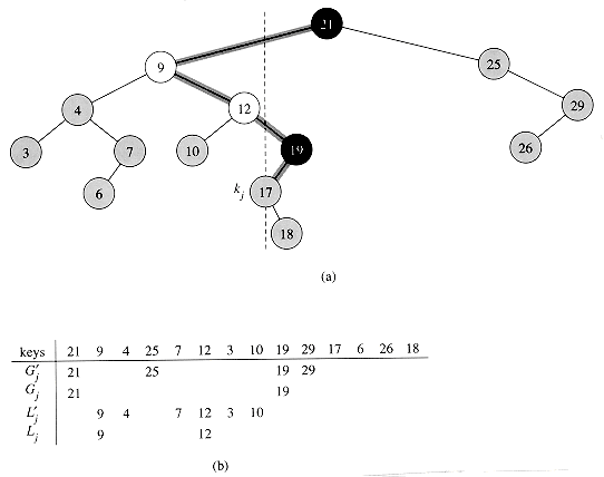
Figure 13.5 illustrates the two sets Gj and Lj. The set Gj contains any key ki inserted before kj such that ki is the smallest key among k1, k2, . . . , ki that is larger than kj. (The structure of Lj is symmetric.) To better understand the set Gj, let us explore a method by which we can enumerate its elements. Among the keys k1, k2, . . . , kj-1, consider in order those that are larger than kj. These keys are shown as G'j, in the figure. As each key is considered in turn, keep a running account of the minimum. The set Gj consists of those elements that update the running minimum.

Let us simplify this scenario somewhat for the purpose of analysis. Suppose that n distinct numbers are inserted one at a time into a dynamic set. If all permutations of the numbers are equally likely, how many times on average does the minimum of the set change? To answer this question, suppose that the ith number inserted is ki, for i = 1, 2, . . . , n. The probability is l/i that ki is the minimum of the first i numbers, since the rank of ki among the first i numbers is equally likely to be any of the i possible ranks. Consequently, the expected number of changes to the minimum of the set is

where Hn = ln n + O(1) is the nth harmonic number (see equation (3.5) and Problem 6-2).

We therefore expect the number of changes to the minimum to be approximately ln n, and the following lemma shows that the probability that it is much greater is very small.

Lemma 13.5

Let k1, k2, . . . , kn be a random permutation of n distinct numbers, and let |S| be the random variable that is the cardinality of the set

S = {ki : 1  i  n and kl > ki for all l < i} .

(13.1)

Then Pr{|S| ( + 1)Hn} 1/n2, where Hn is the nth harmonic number and 4.32 satisfies the equation (ln - 1) = 2.

Proof We can view the cardinality of the set S as being determined by n Bernoulli trials, where a success occurs in the ith trial when ki is smaller than the elements k1, k2, . . . , ki-l. Success in the ith trial occurs with probability 1/i. The trials are independent, since the probability that ki is the minimum of k1, k2, . . . , ki is independent of the relative ordering of k1, k2, . . . , ki-1.

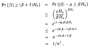
We can use Theorem 6.6 to bound the probability that |S| ( + 1 )Hn . The expectation of |S| is = Hn ln n. Since > 1, Theorem 6.6 yields

Figure 13.5 Illustrating the two sets Gj and Lj that comprise the keys on a path from the root of a binary search tree to a key kj = 17. (a) The nodes with keys in Gj are black, and the nodes with keys in Lj are white. All other nodes are shaded. The path from the root down to the node with key kj is shaded. Keys to the left of the dashed line are less than kj, and keys to the right are greater. The tree is constructed by inserting the keys shown in the topmost list in (b). The set G'j = {21, 25, 19, 29}consists of those elements that are inserted before 17 and are greater than 17. The set Gj = {21, 19} consists of those elements that update a running minimum of the elements in G'j. Thus, the key 21 is in Gj, since it is the first element. The key 25 is not in Gj, since it is larger than the running minimum 21. The key 19 is in Gj, since it is smaller than the running minimum 21. The key 29 is not in Gj, since it is larger than the running minimum 19. The structures of L'j and Lj are symmetric.

which follows from the definition of .

We now have the tools to bound the height of a randomly built binary search tree.

Theorem 13.6

The average height of a randomly built binary search tree on n distinct keys is O(lg n).

Proof Let k1, k2, . . . , kn be a random permutation on the n keys, and let T be the binary search tree that results from inserting the keys in order into an initially empty tree. We first consider the probability that the depth d(kj, T) of a given key kj is at least t, for an arbitrary value t. By the characterization of d (kj, T) in Corollary 13.4, if the depth of kj is at least t, then the cardinality of one of the two sets Gj and Lj must be at least t/2. Thus,

Pr{d(kj, T)  t}  Pr{|Gj|  t/2} + Pr{|Lj|  t/2} .

(13.2)

Let us examine Pr{|Gj|t/2} first. We have

Pr{|Gj|  t/2}

= Pr{|{ki: 1  i < j and kl > ki > kj for all l < i}|  t/2}

 Pr{|{ki: i  n and ki > ki for all l > i}|  t/2}

= Pr{|S|  t/2} ,

where S is defined as in equation (13.1). To justify this argument, note that the probability does not decrease if we extend the range of i from i < j to i n, since more elements are added to the set. Likewise, the probability does not decrease if we remove the condition that ki > kj, since we are substituting a random permutation on possibly fewer than n elements (those ki that are greater than kj) for a random permutation on n elements.

Using a symmetric argument, we can prove that

Pr{|Lj|  t/2}  Pr{|S|  t/2},

and thus, by inequality (13.2), we obtain

Pr {d (kj, T)  t}  2 Pr{|S|  t/2} .

If we choose t = 2( + 1)Hn, where Hn is the nth harmonic number and 4.32 satisfies (1n - l) = 2, we can apply Lemma 13.5 to conclude that

Pr{d(kj, T)  2( + 1)Hn}    2Pr{|S|  ( + 1)Hn}

  2/n2 .

Since there are at most n nodes in a randomly built binary search tree, the probability that any node's depth is at least 2( + 1 )Hn is therefore, by Boole's inequality (6.22), at most n(2/n2) = 2/n. Thus, at least 1 - 2/n of the time, the height of a randomly built binary search tree is less than 2( + 1)Hn, and at most 2/n of the time, it is at most n. The expected height is therefore at most (2( + 1)Hn)(l - 2/n) + n(2/n) = O(lg n).

Exercises

13.4-1

Describe a binary search tree on n nodes such that the average depth of a node in the tree is (lg n) but the height of the tree is w(lg n). How large can the height of an n-node binary search tree be if the average depth of a node is (lg n)?

13.4-2

Show that the notion of a randomly chosen binary search tree on n keys, where each binary search tree of n keys is equally likely to be chosen, is different from the notion of a randomly built binary search tree given in this section. (Hint: List the possibilities when n = 3.)

13.4-3

Given a constant r 1, determine t such that the probability is less than 1 /nr that the height of a randomly built binary search tree is at least tHn.

13.4-4

Consider RANDOMIZED-QUICKSORT operating on a sequence of n input numbers. Prove that for any constant k > 0, all but O(l/nk) of the n! input permutations yield an O(n1g n) running time.

Problems

13-1 Binary search trees with equal keys

Equal keys pose a problem for the implementation of binary search trees.

a. What is the asymptotic performance of TREE-INSERT when used to insert n items with identical keys into an initially empty binary search tree?

We propose to improve TREE-INSERT by testing before line 5 whether or not key[z] = key[x] and by testing before line 11 whether or not key[z] = key[y]. If equality holds, we implement one of the following strategies. For each strategy, find the asymptotic performance of inserting n items with identical keys into an initially empty binary search tree. (The strategies are described for line 5, in which we compare the keys of z and x. Substitute y for x to arrive at the strategies for line 11.)

b. Keep a Boolean flag b[x] at node x, and set x to either left[x] or right[x]based on the value of b[x], which alternates between FALSE and TRUE each time the node is visited during TREE-INSERT.

c. Keep a list of nodes with equal keys at x, and insert z into the list.

d. Randomly set x to either left[x] or right[x]. (Give the worst-case performance and informally derive the average-case performance.)

13-2 Radix trees

Given two strings a = a0a1. . .ap and b = b0b1. . .bq, where each ai and each bj is in some ordered set of characters, we say that string a is lexicographically less than string b if either

1. there exists an integer j, 0 j min(p, q), such that ai = bi for all i = 0, 1, . . . , j - 1 and aj < bj, or

2. p<q and ai = bi for all i = 0, l, . . . , p.

For example, if a and b are bit strings, then 10100 < 10110 by rule 1(letting j = 3) and 10100 < 101000 by rule 2. This is similar to the ordering used in English-language dictionaries.

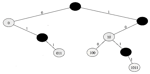
The radix tree data structure shown in Figure 13.6 stores the bit strings 1011, 10, 011, 100, and 0. When searching for a key a = a0a1 . . . ap, we go left at a node of depth i if ai = 0 and right if ai = 1. Let S be a set of distinct binary strings whose lengths sum to n. Show how to use a radix tree to sort S lexicographically in (n) time. For the example in Figure 13.6, the output of the sort should be the sequence 0, 011, 10, 100, 1011.

13-3 Average node depth in a randomly built binary search tree

In this problem, we prove that the average depth of a node in a randomly built binary search tree with n nodes is O(lg n). Although this result is weaker than that of Theorem 13.6, the technique we shall use reveals a surprising similarity between the building of a binary search tree and the running of RANDOMIZED-QUICKSORT from Section 8.3.

We start by recalling from Chapter 5 that the internal path length P(T)of a binary tree T is the sum, over all nodes x in T, of the depth of node x, which we denote by d (x, T).

Figure 13.6 A radix tree storing the bit strings l011, 10, 011, 100, and 0. Each node's key can be determined by traversing the path from the root to that node. There is no need, therefore, to store the keys in the nodes; the keys are shown here for illustrative purposes only. Nodes are heavily shaded if the keys corresponding to them are not in the tree; such nodes are present only to establish a path to other nodes.

a. Argue that the average depth of a node in T is

Thus, we wish to show that the expected value of P(T) is O(n 1g n).

b. Let TL and TR denote the left and right subtrees of tree T, respectively. Argue that if T has n nodes, then

P(T) = P(TL) + P(TR) + n - 1 .

c. Let P(n) denote the average internal path length of a randomly built binary search tree with n nodes. Show that

d. Show that P(n) can be rewritten as

e. Recalling the analysis of the randomized version of quicksort, conclude that P(n) = O(n lg n).

At each recursive invocation of quicksort, we choose a random pivot element to partition the set of elements being sorted. Each node of a binary search tree partitions the set of elements that fall into the subtree rooted at that node.

f. Describe an implementation of quicksort in which the comparisons to sort a set of elements are exactly the same as the comparisons to insert the elements into a binary search tree. (The order in which comparisons are made may differ, but the same comparisons must be made.)

13-4 Number of different binary trees

Let bn denote the number of different binary trees with n nodes. In this problem, you will find a formula for bn as well as an asymptotic estimate.

a. Show that b0 = 1 and that, for n 1,

b Let B(x) be the generating function

(see Problem 4-6 for the definition of generating functions). Show that B(x) = xB(x)2 + 1 and hence

The Taylor expansion of f(x) around the point x = a is given by

where f(k) (x) is the kth derivative of f evaluated at x.

c. Show that

(the nth Catalan number) by using the Taylor expansion of around x = 0. (If you wish, instead of using the Taylor expansion, you may use the generalization of the binomial expansion (6.5) to non-integral exponents n, where for any real number n and integer k, we interpret to be n(n - 1) . . . (n - k + 1)/k! if k 0, and 0 otherwise.)

d. Show that

Chapter notes

Knuth [123] contains a good discussion of simple binary search trees as well as many variations. Binary search trees seem to have been independently discovered by a number of people in the late 1950's.

Go to Chapter 14     Back to Table of Contents