 (n2) on an input array of n numbers. In spite of this slow worst-case running time, quicksort is often the best practical choice for sorting because it is remarkably efficient on the average: its expected running time is
  (n lg n), and the constant factors hidden in the
  (n lg n) notation are quite small. It also has the advantage of sorting in place (see page 3), and it works well even in virtual memory environments.
Section 8.1 describes the algorithm and an important subroutine used by quicksort for partitioning. Because the behavior of quicksort is complex, we start with an intuitive discussion of its performance in Section 8.2 and postpone its precise analysis to the end of the chapter. Section 8.3 presents two versions of quicksort that use a random-number generator. These "randomized" algorithms have many desirable properties. Their average-case running time is good, and no particular input elicits their worst-case behavior. One of the randomized versions of quicksort is analyzed in Section 8.4, where it is shown to run in O(n2) time in the worst case and in O(n lg n) time on average.
8.1 Description of quicksort
Quicksort, like merge sort, is based on the divide-and-conquer paradigm introduced in Section 1.3.1. Here is the three-step divide-and-conquer process for sorting a typical subarray A[p . . r].
Divide: The array A[p . . r] is partitioned (rearranged) into two nonempty subarrays A[p . . q] and A[q + 1 . . r] such that each element of A[p . . q] is less than or equal to each element of A[q + 1 . . r]. The index q is computed as part of this partitioning procedure.
Conquer: The two subarrays A[p . . q] and A[q + 1 . . r] are sorted by recursive calls to quicksort.
Combine: Since the subarrays are sorted in place, no work is needed to combine them: the entire array A[p . . r] is now sorted.
The following procedure implements quicksort.
To sort an entire array A, the initial call is QUICKSORT(A, 1, length[A]).
The key to the algorithm is the PARTITION procedure, which rearranges the subarray A[p . . r] in place.
Figure 8.1 shows how PARTITION works. It first selects an element x = A[p] from A[p . . r] as a "pivot" element around which to partition A[p . . r]. It then grows two regions A[p . . i] and A[j . . r] from the top and bottom of A[p . . r], respectively, such that every element in A[p . . i] is less than or equal to x and every element in A[j . . r] is greater than or equal to x. Initially, i = p - 1 and j = r + 1, so the two regions are empty.
Within the body of the while loop, the index j is decremented and the index i is incremented, in lines 5-8, until A[i]
The body of the while loop repeats until i
Conceptually, the partitioning procedure performs a simple function: it puts elements smaller than x into the bottom region of the array and elements larger than x into the top region. There are technicalities that make the pseudocode of PARTITION a little tricky, however. For example, the indices i and j never index the subarray A[p . . r] out of bounds, but this isn't entirely apparent from the code. As another example, it is important that A[p] be used as the pivot element x. If A[r] is used instead and it happens that A[r] is also the largest element in the subarray A[p . . r], then PARTITION returns to QUICKSORT the value q = r, and QUICKSORT loops forever. Problem 8-1 asks you to prove PARTITION correct.
The running time of PARTITION on an array A[p . . r] is
8.1-1
Using Figure 8.1 as a model, illustrate the operation of PARTITION on the array A =
8.1-2
What value of q does PARTITION return when all elements in the array A[p . . r] have the same value?
8.1-3
Give a brief argument that the running time of PARTITION on a subarray of size n is
8.1-4
How would you modify QUICKSORT to sort in nonincreasing order?
The running time of quicksort depends on whether the partitioning is balanced or unbalanced, and this in turn depends on which elements are used for partitioning. If the partitioning is balanced, the algorithm runs asymptotically as fast as merge sort. If the partitioning is unbalanced, however, it can run asymptotically as slow as insertion sort. In this section, we shall informally investigate how quicksort performs under the assumptions of balanced versus unbalanced partitioning.
The worst-case behavior for quicksort occurs when the partitioning routine produces one region with n - 1 elements and one with only l element. (This claim is proved in Section 8.4.1.) Let us assume that this unbalanced partitioning arises at every step of the algorithm. Since partitioning costs
To evaluate this recurrence, we observe that T(1) =
We obtain the last line by observing that
Thus, if the partitioning is maximally unbalanced at every recursive step of the algorithm, the running time is
If the partitioning procedure produces two regions of size n/2, quicksort runs much faster. The recurrence is then
which by case 2 of the master theorem (Theorem 4.1) has solution T(n) =
The average-case running time of quicksort is much closer to the best case than to the worst case, as the analyses in Section 8.4 will show. The key to understanding why this might be true is to understand how the balance of the partitioning is reflected in the recurrence that describes the running time.
Suppose, for example, that the partitioning algorithm always produces a 9-to-1 proportional split, which at first blush seems quite unbalanced. We then obtain the recurrence
on the running time of quicksort, where we have replaced
To develop a clear notion of the average case for quicksort, we must make an assumption about how frequently we expect to encounter the various inputs. A common assumption is that all permutations of the input numbers are equally likely. We shall discuss this assumption in the next section, but first let's explore its ramifications.
When we run quicksort on a random input array, it is unlikely that the partitioning always happens in the same way at every level, as our informal analysis has assumed. We expect that some of the splits will be reasonably well balanced and that some will be fairly unbalanced. For example, Exercise 8.2-5 asks to you show that about 80 percent of the time PARTITION produces a split that is more balanced than 9 to 1, and about 20 percent of the time it produces a split that is less balanced than 9 to 1.
In the average case, PARTITION produces a mix of "good" and "bad" splits. In a recursion tree for an average-case execution of PARTITION, the good and bad splits are distributed randomly throughout the tree. Suppose for the sake of intuition, however, that the good and bad splits alternate levels in the tree, and that the good splits are best-case splits and the bad splits are worst-case splits. Figure 8.5(a) shows the splits at two consecutive levels in the recursion tree. At the root of the tree, the cost is n for partitioning and the subarrays produced have sizes n - 1 and 1: the worst case. At the next level, the subarray of size n - 1 is best-case partitioned into two subarrays of size (n - 1)/2. Let's assume that the boundary-condition cost is 1 for the subarray of size 1.
The combination of the bad split followed by the good split produces three subarrays of sizes 1, (n -1)/2, and (n - 1)/2 at a combined cost of 2n - 1 =
8.2-1
Show that the running time of QUICKSORT is
8.2-2
Show that the running time of QUICKSORT is
8.2-3
Banks often record transactions on an account in order of the times of the transactions, but many people like to receive their bank statements with checks listed in order by check number. People usually write checks in order by check number, and merchants usually cash them with reasonable dispatch. The problem of converting time-of-transaction ordering to check-number ordering is therefore the problem of sorting almost-sorted input. Argue that the procedure INSERTION-SORT would tend to beat the procedure QUICKSORT on this problem.
8.2-4
Suppose that the splits at every level of quicksort are in the proportion 1 -
8.2-5
Argue that for any constant 0 <
In exploring the average-case behavior of quicksort, we have made an assumption that all permutations of the input numbers are equally likely. When this assumption on the distribution of the inputs is valid, many people regard quicksort as the algorithm of choice for large enough inputs. In an engineering situation, however, we cannot always expect it to hold. (See Exercise 8.2-3.) This section introduces the notion of a randomized algorithm and presents two randomized versions of quicksort that overcome the assumption that all permutations of the input numbers are equally likely.
An alternative to assuming a distribution of inputs is to impose a distribution. For example, suppose that before sorting the input array, quicksort randomly permutes the elements to enforce the property that every permutation is equally likely. (Exercise 8.3-4 asks for an algorithm that randomly permutes the elements of an array of size n in time O(n).) This modification does not improve the worst-case running time of the algorithm, but it does make the running time independent of the input ordering.
We call an algorithm randomized if its behavior is determined not only by the input but also by values produced by a random-number generator. We shall assume that we have at our disposal a random-number generator RANDOM. A call to RANDOM(a,b) returns an integer between a and b, inclusive, with each such integer being equally likely. For example, RANDOM(0, 1) produces a 0 with probability 1/2 and a 1 with probability 1/2. Each integer returned by RANDOM is independent of the integers returned on previous calls. You may imagine RANDOM as rolling a (b - a + 1 )-sided die to obtain its output. (In practice, most programming environments offer a pseudorandom-number generator: a deterministic algorithm that returns numbers that "look" statistically random.)
This randomized version of quicksort has an interesting property that is also possessed by many other randomized algorithms: no particular input elicits its worst-case behavior. Instead, its worst case depends on the random-number generator. Even intentionally, you cannot produce a bad input array for quicksort, since the random permutation makes the input order irrelevant. The randomized algorithm performs badly only if the random-number generator produces an unlucky permutation to be sorted. Exercise 13.4-4 shows that almost all permutations cause quicksort to perform nearly as well as the average case: there are very few permutations that cause near-worst-case behavior.
A randomized strategy is typically useful when there are many ways in which an algorithm can proceed but it is difficult to determine a way that is guaranteed to be good. If many of the alternatives are good, simply choosing one randomly can yield a good strategy. Often, an algorithm must make many choices during its execution. If the benefits of good choices outweigh the costs of bad choices, a random selection of good and bad choices can yield an efficient algorithm. We noted in Section 8.2 that a mixture of good and bad splits yields a good running time for quicksort, and thus it makes sense that randomized versions of the algorithm should perform well.
By modifying the PARTITION procedure, we can design another randomized version of quicksort that uses this random-choice strategy. At each step of the quicksort algorithm, before the array is partitioned, we exchange element A[p] with an element chosen at random from A[p . . r]. This modification ensures that the pivot element x = A[p] is equally likely to be any of the r - p + 1 elements in the subarray. Thus, we expect the split of the input array to be reasonably well balanced on average. The randomized algorithm based on randomly permuting the input array also works well on average, but it is somewhat more difficult to analyze than this version.
The changes to PARTITION and QUICKSORT are small. In the new partition procedure, we simply implement the swap before actually partitioning:
We now make the new quicksort call RANDOMIZED-PARTITION in place of PARTITION:
We analyze this algorithm in the next section.
8.3-1
Why do we analyze the average-case performance of a randomized algorithm and not its worst-case performance?
8.3-2
During the running of the procedure RANDOMIZED-QUICKSORT, how many calls are made to the random-number generator RANDOM in the worst case? How does the answer change in the best case?
8.3-3
Describe an implementation of the procedure RANDOM(a, b) that uses only fair coin flips. What is the expected running time of your procedure?
8.3-4
Give a
Section 8.2 gave some intuition for the worst-case behavior of quicksort and for why we expect it to run quickly. In this section, we analyze the behavior of quicksort more rigorously. We begin with a worst-case analysis, which applies to either QUICKSORT or RANDOMIZED-QUICKSORT, and conclude with an average-case analysis of RANDOMIZED-QUICKSORT.
We saw in Section 8.2 that a worst-case split at every level of recursion in quicksort produces a
Using the substitution method (see Section 4.1), we can show that the running time of quicksort is O(n2). Let T(n) be the worst-case time for the procedure QUICKSORT on an input of size n. We have the recurrence
where the parameter q ranges from 1 to n - 1 because the procedure PARTITION produces two regions, each having size at least 1. We guess that T(n)
The expression q2 + (n - q)2 achieves a maximum over the range 1
Continuing with our bounding of T(n), we obtain
since we can pick the constant c large enough so that the 2c(n - 1) term dominates the
We have already given an intuitive argument why the average-case running time of RANDOMIZED-QUICKSORT is
We first make some observations about the operation of PARTITION. When PARTITION is called in line 3 of the procedure RANDOMIZED-PARTITION, the element A[p] has already been exchanged with a random element in A[p . . r]. To simplify the analysis, we assume that all input numbers are distinct. If all input numbers are not distinct, it is still true that quick-sort's average-case running time is O(n lg n), but a somewhat more intricate analysis than we present here is required.
Our first observation is that the value of q returned by PARTITION depends only on the rank of x = A[p] among the elements in A[p . . r]. (The rank of a number in a set is the number of elements less than or equal to it.) If we let n = r - p + 1 be the number of elements in A[p . . r], swapping A[p] with a random element from A[p . . r] yields a probability 1/n that rank(x) = i for i = 1,2, . . . , n.
We next compute the likelihoods of the various outcomes of the partitioning. If rank(x) = 1, then the first time through the while loop in lines 4-11 of PARTITION, index i stops at i = p and index j stops at j = p. Thus, when q = j is returned, the "low" side of the partition contains the sole element A[p]. This event occurs with probability 1/n since that is the probability that rank(x) = 1.
If rank(x)
Combining these two cases, we conclude that the size q - p + 1 of the low side of the partition is 1 with probability 2/n and that the size is i with probability 1 /n for i = 2,3, . . . , n - 1.
We now establish a recurrence for the expected running time of RANDOMIZED-QUICKSORT. Let T(n) denote the average time required to sort an n-element input array. A call to RANDOMIZED-QUICKSORT with a 1-element array takes constant time, so we have T(1) =
The value of q has an almost uniform distribution, except that the value q = 1 is twice as likely as the others, as was noted above. Using the facts that T(1) =
and the term
Observe that for k = 1,2, . . . , n - 1, each term T(k) of the sum occurs once as T(q) and once as T(n - q). Collapsing the two terms of the sum yields
We can solve the recurrence (8.4) using the substitution method. Assume inductively that T(n)
We show below that the summation in the last line can be bounded by
Using this bound, we obtain
since we can choose a large enough so that
It remains to prove the bound (8.5) on the summation
Since each term is at most n lg n, we have the bound
which is tight to within a constant factor. This bound is not strong enough to solve the recurrence as T(n) = O(n lg n), however. Specifically, we need a bound of
We can get this bound on the summation by splitting it into two parts, as discussed in Section 3.2 on page 48. We obtain
The lg k in the first summation on the right is bounded above by 1g(n/2) = 1g n - 1. The lg k in the second summation is bounded above by lg n. Thus,
if n
8.4-1
Show that quicksort's best-case running time is
8.4-2
Show that q2 + (n - q)2 achieves a maximum over q = 1, 2, . . . , n - 1 when q = 1 or q = n - 1.
8.4-3
Show that RANDOMIZED-QUICKSORT's expected running time is
8.4-4
The running time of quicksort can be improved in practice by taking advantage of the fast running time of insertion sort when its input is "nearly" sorted. When quicksort is called on a subarray with fewer than k elements, let it simply return without sorting the subarray. After the top-level call to quicksort returns, run insertion sort on the entire array to finish the sorting process. Argue that this sorting algorithm runs in O(nk + n 1g(n/k)) expected time. How should k be picked, both in theory and in practice?
8.4-5
Prove the identity
and then use the integral approximation method to give a tighter upper bound than (8.5) on the summation
8.4-6
Consider modifying the PARTITION procedure by randomly picking three elements from array A and partitioning about their median. Approximate the probability of getting at worst an
8-1 Partition correctness
Give a careful argument that the procedure PARTITION in Section 8.1 is correct. Prove the following:
a. The indices i and j never reference an element of A outside the interval [p . . r].
b. The index j is not equal to r when PARTITION terminates (so that the split is always nontrivial).
c. Every element of A[p . . j] is less than or equal to every element of A[j+ 1 . . r] when PARTITION terminates.
8-2 Lomuto's partitioning algorithm
Consider the following variation of PARTITION, due to N. Lomuto. To partition A[p . . r], this version grows two regions, A[p . . i] and A[i + 1 . . j], such that every element in the first region is less than or equal to x = A [r] and every element in the second region is greater than x.
a. Argue that LOMUTO-PARTITION is correct.
b. What are the maximum numbers of times that an element can be moved by PARTITION and by LOMUTO-PARTITION?
c. Argue that LOMUTO-PARTITION, like PARTITION, runs in
d. How does replacing PARTITION by LOMUTO-PARTITION affect the running time of QUICKSORT when all input values are equal?
e. Define a procedure RANDOMIZED-LOMUTO-PARTITION that exchanges A[r] with a randomly chosen element in A[p . . r] and then calls LOMUTO-PARTITION. Show that the probability that a given value q is returned by RANDOMIZED-LOMUTO-PARTITION is equal to the probability that p + r - q is returned by RANDOMIZED-PARTITION.
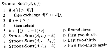
8-3 Stooge sort
Professors Howard, Fine, and Howard have proposed the following "elegan" sorting algorithm:
a. Argue that STOOGE-SORT(A, 1, length[A]) correctly sorts the input array A[1 . . n], where n = length[A].
b. Give a recurrence for the worst-case running time of STOOGE-SORT and a tight asymptotic (
c. Compare the worst-case running time of STOOGE-SORT with that of insertion sort, merge sort, heapsort, and quicksort. Do the professors deserve tenure?
8-4 Stack depth for quicksort
The QUICKSORT algorithm of Section 8.1 contains two recursive calls to itself. After the call to PARTITION, the left subarray is recursively sorted and then the right subarray is recursively sorted. The second recursive call in QUICKSORT is not really necessary; it can be avoided by using an iterative control structure. This technique, called tail recursion, is provided automatically by good compilers. Consider the following version of quicksort, which simulates tail recursion.
a. Argue that QUICKSORT'(A, 1, length[A]) correctly sorts the array A.
Compilers usually execute recursive procedures by using a stack that contains pertinent information, including the parameter values, for each recursive call. The information for the most recent call is at the top of the stack, and the information for the initial call is at the bottom. When a procedure is invoked, its information is pushed onto the stack; when it terminates, its information is popped. Since we assume that array parameters are actually represented by pointers, the information for each procedure call on the stack requires O(1) stack space. The stack depth is the maximum amount of stack space used at any time during a computation.
b. Describe a scenario in which the stack depth of QUICKSORT' is
c. Modify the code for QUICKSORT' so that the worst-case stack depth is
8-5 Median-of-3 partition
One way to improve the RANDOMIZED-QUICKSORT procedure is to partition around an element x that is chosen more carefully than by picking a random element from the subarray. One common approach is the median-of-3 method: choose x as the median (middle element) of a set of 3 elements randomly selected from the subarray. For this problem, let us assume that the elements in the input array A[1 . . n] are distinct and that n
a. Give an exact formula for pi as a function of n and i for i = 2, 3, . . . , n - 1 . (Note that p1 = pn = 0.)
b. By what amount have we increased the likelihood of choosing x = A'[
c. If we define a "good" split to mean choosing x = A'[i], where n/3
d. Argue that the median-of-3 method affects only the constant factor in the
The quicksort procedure was invented by Hoare [98]. Sedgewick [174] provides a good reference on the details of implementation and how they matter. The advantages of randomized algorithms were articulated by Rabin [165].
QUICKSORT(A,p,r)
1 if p < r
2 then q
 PARTITION(A,p,r)
3 QUICKSORT(A,p,q)
4 QUICKSORT(A,q + 1,r)
Partitioning the array
PARTITION(A,p,r)
1 x
 A[p]
A[p]2 i
 p - 1
p - 13 j
 r + 1
r + 14 while TRUE
5 do repeat j
 j - 1
j - 16 until A[j]
 x
x7 repeat i
 i + 1
i + 18 until A[i]
 x
x9 if i < j
10 then exchange A[i]
 A[j]
A[j]11 else return j
 x
x  A[j]. Assuming that these inequalities are strict, A[i] is too large to belong to the bottom region and A[j] is too small to belong to the top region. Thus, by exchanging A[i] and A[j] as is done in line 10, we can extend the two regions. (If the inequalities are not strict, the exchange can be performed anyway.)
 j, at which point the entire array A[p . . r] has been partitioned into two subarrays A[p . . q] and A[q + 1 . . r], where p
  q < r, such that no element of A[p . . q] is larger than any element of A[q + 1. . r]. The value q = j is returned at the end of the procedure.
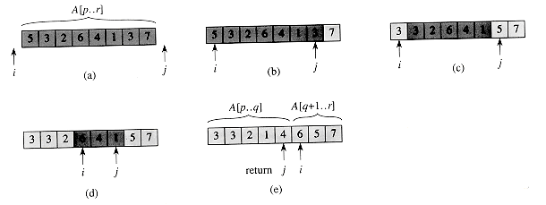
Figure 8.1 The operation of PARTITION on a sample array. Lightly shaded array elements have been placed into the correct partitions, and heavily shaded elements are not yet in their partitions. (a) The input array, with the initial values of i and j just off the left and right ends of the array. We partition around x = A[p] = 5. (b) The positions of i and j at line 9 of the first iteration of the while loop. (c) The result of exchanging the elements pointed to by i and j in line 10. (d) The positions of i and j at line 9 of the second iteration of the while loop. (e) The positions of i and j at line 9 of the third and last iteration of the while loop. The procedure terminates because i
 j, and the value q = j is returned. Array elements up to and including A[j] are less than or equal to x = 5, and array elements after A[j] are greater than or equal to x = 5.
 (n), where n = r - p + 1 (see Exercise 8.1-3).
Exercises
 13, 19, 9, 5, 12, 8, 7, 4, 11, 2, 6, 21
 .
. (n).
(n).8.2 Performance of quicksort
Worst-case partitioning
 (n) time and T(1) =
  (1), the recurrence for the running time is
T(n) = T(n - 1) +
 (n).
(n). (1) and then iterate:
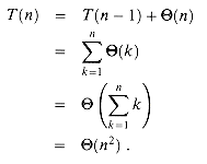
 is the arithmetic series (3.2). Figure 8.2 shows a recursion tree for this worst-case execution of quicksort. (See Section 4.2 for a discussion of recursion trees.)
 (n2). Therefore the worstcase running time of quicksort is no better than that of insertion sort. Moreover, the
  (n2) running time occurs when the input array is already completely sorted--a common situation in which insertion sort runs in O(n) time.
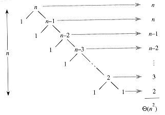
Figure 8.2 A recursion tree for QUICKSORT in which the PARTITION procedure always puts only a single element on one side of the partition (the worst case). The resulting running time is
 (n2).
(n2).Best-case partitioning
T(n) = 2T(n/2) +
 (n),
(n), (n lg n). Thus, this best-case partitioning produces a much faster algorithm. Figure 8.3 shows the recursion tree for this best-case execution of quicksort.
Balanced partitioning
T(n) = T(9n/10) + T(n/10) + n
 (n) by n for convenience. Figure 8.4 shows the recursion tree for this recurrence. Notice that every level of the tree has cost n, until a boundary condition is reached at depth log10 n =
  (lg n), and then the levels have cost at most n. The recursion terminates at depth log10/9 n =
  (lg n). The total cost of quicksort is therefore
  (n lg n). Thus, with a 9-to-1 proportional split at every level of recursion, which intuitively seems quite unbalanced, quicksort runs in
  (n lg n) time--asymptotically the same as if the split were right down the middle. In fact, even a 99-to-1 split yields an O(n lg n) running time. The reason is that any split of constant proportionality yields a recursion tree of depth
  (lg n), where the cost at each level is O(n). The running time is therefore
  (n lg n) whenever the split has constant proportionality.
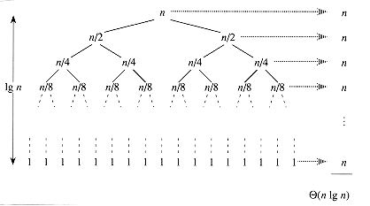
Figure 8.3 A recursion tree for QUICKSORT in which PARTITION always balances the two sides of the partition equally (the best case). The resulting running time is
 (n lg n).
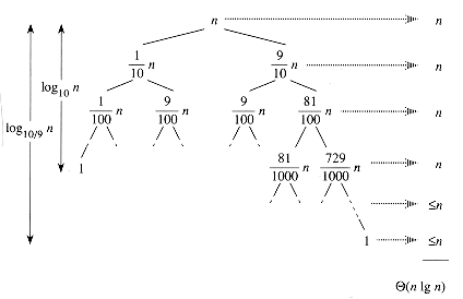
Figure 8.4 A recursion tree for QUICKSORT in which PARTITION always produces a 9-to-1 split, yielding a running time of
 (n lg n).
Intuition for the average case
 (n). Certainly, this situation is no worse than that in Figure 8. 5 (b), namely a single level of partitioning that produces two subarrays of sizes (n - 1)/2 + 1 and (n - 1)/2 at a cost of n =
  (n). Yet this latter situation is very nearly balanced, certainly better than 9 to 1. Intuitively, the
  (n) cost of the bad split can be absorbed into the
  (n) cost of the good split, and the resulting split is good. Thus, the running time of quicksort, when levels alternate between good and bad splits, is like the running time for good splits alone: still O(n lg n), but with a slightly larger constant hidden by the O-notation. We shall give a rigorous analysis of the average case in Section 8.4.2.
Figure 8.5 (a) Two levels of a recursion tree for quicksort. The partitioning at the root costs n and produces a "bad" split: two subarrays of sizes 1 and n - 1. The partitioning of the subarray of size n - 1 costs n - 1 and produces a "good" split: two subarrays of size (n - 1)/2. (b) A single level of a recursion tree that is worse than the combined levels in (a), yet very well balanced.
Exercises
 (n lg n) when all elements of array A have the same value.
 (n2) when the array A is sorted in nonincreasing order.
 to
to  , where 0 <
 1/2 is a constant. Show that the minimum depth of a leaf in the recursion tree is approximately ep1g n/lg
  and the maximum depth is approximately - lg n/lg(1 -
  ). (Don't worry about integer round-off.)
 1/2, the probability is approximately 1 - 2
 that on a random input array, PARTITION produces a split more balanced than 1 -
  to
to  . For what value of
  are the odds even that the split is more balanced than less balanced?
8.3 Randomized versions of quicksort
RANDOMIZED-PARTITION(A,p,r)
1 i
 RANDOM(p,r)
2 exchange A[p]
 A[i]
A[i]3 return PARTITION(A,p,r)
RANDOMIZED-QUICKSORT(A,p,r)
1 if p < r
2 then q
 RANDOMIZED-PARTITION(A,p,r)
3 RANDOMIZED-QUICKSORT(A,p,q)
4 RANDOMIZED-QUICKSORT(A,q + 1,r)
Exercises
 (n)-time, randomized procedure that takes as input an array A[1 . . n] and performs a random permutation on the array elements.
8.4 Analysis of quicksort
8.4.1 Worst-case analysis
 (n2) running time, which, intuitively, is the worst-case running time of the algorithm. We now prove this assertion.
(8.1)
 cn2 for some constant c. Substituting this guess into (8.1), we obtain
 q
q  n - 1 at one of the endpoints, as can be seen since the second derivative of the expression with respect to q is positive (see Exercise 8.4-2). This gives us the bound max1
 q
q n - 1(q2 + (n - q)2)
  12 + (n - 1)2 = n2 - 2(n - 1).
T(n)
 cn2 - 2c(n - 1) +
  (n)
(n) cn2 ,
cn2 , (n) term. Thus, the (worst-case) running time of quicksort is
  (n2).
(n2).8.4.2 Average-case analysis
 (n 1g n): if the split induced by RANDOMIZED-PARTITION puts any constant fraction of the elements on one side of the partition, then the recursion tree has depth
  (1g n) and
  (n) work is performed at
  (1g n) of these levels. We can analyze the expected running time of RANDOMIZED-QUICKSORT precisely by first understanding how the partitioning procedure operates. We can then develop a recurrence for the average time required to sort an n-element array and solve this recurrence to determine bounds on the expected running time. As part of the process of solving the recurrence, we shall develop tight bounds on an interesting summation.
Analysis of partitioning
 2, then there is at least one element smaller than x = A[p]. Consequently, the first time through the while loop, index i stops at i = p but j stops before reaching p. An exchange with A[p] is then made to put A[p] in the high side of the partition. When PARTITION terminates, each of the rank(x) - 1 elements in the low side of the partition is strictly less than x. Thus, for each i = 1,2, . . . , n - l, when rank(x)
  2, the probability is 1/n that the low side of the partition has i elements.
A recurence for the average case
 (1). A call to RANDOMIZED-QUICKSORT with an array A[l . . n] of length n uses time
  (n) to partition the array. The PARTITION procedure returns an index q, and then RANDOMIZED-QUICKSORT is called recursively with subarrays of length q and n - q. Consequently, the average time to sort an array of length n can be expressed as
(8.2)
 (1) and T(n - 1) = O(n2) from our worst-case analysis, we have
 (n) in equation (8.2) can therefore absorb the expression
  . We can thus restate recurrence (8.2) as
(8.3)

(8.4)
Solving the recurrence
 an 1g n + b for some constants a > 0 and b > 0 to be determined. We can pick a and b sufficiently large so that an 1g n + b is greater than T(1). Then for n > 1, we have by substitution
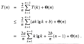

(8.5)
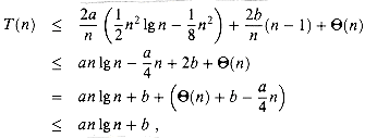
 dominates
  (n) + b. We conclude that quicksort's average running time is O(n lg n).
Tight bounds on the key summation


 for the solution of the recurrence to work out.
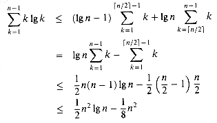
 2. This is the bound (8.5).
Exercises
 (n1gn).
 (n 1g n).
 .
. -to-(1 -
  ) split, as a function of
  in the range 0 <
  < 1.
< 1.Problems
LOMUTO-PARTITION(A, p, r)
1 x
 A[r]
A[r]2 i
 p - 1
p - 13 for j
 p to r
4 do if A[j]
 x
x5 then i
 i + 1
i + 16 exchange A[i]
 A[j]
A[j]7 if i < r
8 then return i
9 else return i - 1
 (n) time on an n-element subarray.
 -notation) bound on the worst-case running time.
QUICKSORT'(A,p,r)
1 while p < r
2 do
 Partition and sort left subarray
3 q
 PARTITION(A,p,r)
4 QUICKSORT'(A,p,q)
5 p
 q + 1
q + 1 (n) on an n-element input array.
 (1g n).
 3. We denote the sorted output array by A'[1 . . n]. Using the median-of-3 method to choose the pivot element x, define pi = Pr{x = A'[i]}.
 (n + 1)/2
 ], the median of A[1 . . n], compared to the ordinary implementation? Assume that n
 , and give the limiting ratio of these probabilities.
 i
i  2n/3, by what amount have we increased the likelihood of getting a good split compared to the ordinary implementation? (Hint: Approximate the sum by an integral.)
 (n 1g n) running time of quicksort.
Chapter notes


