6.1 Counting
Counting theory tries to answer the question "How many?" without actually enumerating how many. For example, we might ask, "How many different n-bit numbers are there?" or "How many orderings of n distinct elements are there?" In this section, we review the elements of counting theory. Since some of the material assumes a basic understanding of sets, the reader is advised to start by reviewing the material in Section 5.1.
Rules of sum and product
A set of items that we wish to count can sometimes be expressed as a union of disjoint sets or as a Cartesian product of sets.
The rule of sum says that the number of ways to choose an element from one of two disjoint sets is the sum of the cardinalities of the sets.That is, if A and B are two finite sets with no members in common, then |A
The rule of product says that the number of ways to choose an ordered pair is the number of ways to choose the first element times the number of ways to choose the second element. That is, if A and B are two finite sets, then |A
A string over a finite set S is a sequence of elements of S. For example, there are 8 binary strings of length 3:
We sometimes call a string of length k a k-string. A substring s' of a string s is an ordered sequence of consecutive elements of s. A k-substring of a string is a substring of length k. For example, 010 is a 3-substring of 01101001 (the 3-substring that begins in position 4), but 111 is not a substring of 01101001.
A k-string over a set S can be viewed as an element of the Cartesian product Sk of k-tuples; thus, there are |S|k strings of length k. For example, the number of binary k-strings is 2k. Intuitively, to construct a k-string over an n-set, we have n ways to pick the first element; for each of these choices, we have n ways to pick the second element; and so forth k times. This construction leads to the k-fold product n
A permutation of a finite set S is an ordered sequence of all the elements of S, with each element appearing exactly once. For example, if S = {a, b, c}, there are 6 permutations of S:
There are n! permutations of a set of n elements, since the first element of the sequence can be chosen in n ways, the second in n - 1 ways, the third in n - 2 ways, and so on.
A k-permutation of S is an ordered sequence of k elements of S, with no element appearing more than once in the sequence. (Thus, an ordinary permutation is just an n-permutation of an n-set.) The twelve 2-permutations of the set {a, b, c, d} are
The number of k-permutations of an n-set is
since there are n ways of choosing the first element, n - 1 ways of choosing the second element, and so on until k elements are selected, the last being a selection from n - k + 1 elements.
A k-combination of an n-set S is simply a k-subset of S. There are six 2-combinations of the 4-set {a, b, c, d}:
(Here we use the shorthand of denoting the 2-set {a,b} by ab, and so on.) We can construct a k-combination of an n-set by choosing k distinct (different) elements from the n-set.
The number of k-combinations of an n-set can be expressed in terms of the number of k-permutations of an n-set. For every k-combination, there are exactly k! permutations of its elements, each of which is a distinct k-permutation of the n-set. Thus, the number of k-combinations of an n-set is the number of k-permutations divided by k!; from equation (6.1), this quantity is
For k = 0, this formula tells us that the number of ways to choose 0 elements from an n-set is 1 (not 0), since 0! = 1.
We use the notation
This formula is symmetric in k and n - k:
These numbers are also known as binomial coefficients, due to their appearance in the binomial expansion:
A special case of the binomial expansion occurs when x = y = 1:
This formula corresponds to counting the 2n binary n-strings by the number of 1's they contain: there are
There are many identities involving binomial coefficients. The exercises at the end of this section give you the opportunity to prove a few.
We sometimes need to bound the size of a binomial coefficient. For 1
Taking advantage of the inequality k!
For all 0
where for convenience we assume that 00 = 1. For k =
where
is the (binary) entropy function and where, for convenience, we assume that 0 lg 0 = 0, so that H (0) = H (1) = 0.
6.1-1
How many k-substrings does an n-string have? (Consider identical k-substrings at different positions as different.) How many substrings does an n-string have in total?
6.1-2
An n-input, m-output boolean function is a function from {TRUE, FALSE}n to {TRUE, FALSE}m. How many n-input, 1-output boolean functions are there? How many n-input, m-output boolean functions are there?
6.1-3
In how many ways can n professors sit around a circular conference table? Consider two seatings to be the same if one can be rotated to form the other.
6.1-4
In how many ways can three distinct numbers be chosen from the set {1, 2, . . . , 100} so that their sum is even?
6.1-5
Prove the identity
for 0 < k
6.1-6
Prove the identity
for 0
6.1-7
To choose k objects from n, you can make one of the objects distinguished and consider whether the distinguished object is chosen. Use this approach to prove that
6.1-8
Using the result of Exercise 6.1-7, make a table for n = 0, 1, . . . , 6 and 0
6.1-9
Prove that
6.1-10
Show that for any n
6.1-11
Argue that for any n
**image 104_g.gif not available**
Provide both an algebraic proof and an argument based on a method for choosing j + k items out of n. Give an example in which equality does not hold.
6.1-12
Use induction on k
6.1-13
Use Stirling's approximation to prove that
**image 104_h.gif not available**
6.1-14
By differentiating the entropy function H (
Probability is an essential tool for the design and analysis of probabilistic and randomized algorithms. This section reviews basic probability theory.
We define probability in terms of a sample space S, which is a set whose elements are called elementary events. Each elementary event can be viewed as a possible outcome of an experiment. For the experiment of flipping two distinguishable coins, we can view the sample space as consisting of the set of all possible 2-strings over {H, T}:
An event is a subset1 of the sample space S. For example, in the experiment of flipping two coins, the event of obtaining one head and one tail is {HT, TH}. The event S is called the certain event, and the event
1 For a general probability distribution, there may be some subsets of the sample space S that are not considered to be events. This situation usually arises when the sample space is uncountably infinite. The main requirement is that the set of events of a sample space be closed under the operations of taking the complement of an event, forming the union of a finite or countable number of events, and taking the intersection of a finite or countable number of events. Most of the probability distributions we shall see are over finite or countable sample spaces, and we shall generally consider all subsets of a sample space to be events. A notable exception is the continuous uniform probability distribution, which will be presented shortly.
A probability distribution Pr{} on a sample space S is a mapping from events of S to real numbers such that the following probability axioms are satisfied:
1. Pr {A}
2. Pr {S} = 1.
3. Pr {A
We call Pr {A} the probability of the event A. We note here that axiom 2 is a normalization requirement: there is really nothing fundamental about choosing 1 as the probability of the certain event, except that it is natural and convenient.
Several results follow immediately from these axioms and basic set theory (see Section 5.1). The null event
In our coin-flipping example, suppose that each of the four elementary events has probability 1/4. Then the probability of getting at least one head is
Alternatively, since the probability of getting strictly less than one head is Pr{TT} = 1/4, the probability of getting at least one head is 1 - 1/4 = 3/4.
A probability distribution is discrete if it is defined over a finite or countably infinite sample space. Let S be the sample space. Then for any event A,
since elementary events, specifically those in A, are mutually exclusive. If S is finite and every elementary event s
then we have the uniform probability distribution on S. In such a case the experiment is often described as "picking an element of S at random."
As an example, consider the process of flipping a fair coin, one for which the probability of obtaining a head is the same as the probability of obtaining a tail, that is, 1/2. If we flip the coin n times,we have the uniform probability distribution defined on the sample space S = {H, T}n, a set of size 2n. Each elementary event in S can be represented as a string of length n over {H, T}, and each occurs with probability 1/2n. The event
is a subset of S of size
The continuous uniform probability distribution is an example of a probability distribution in which all subsets of the sample space are not considered to be events. The continuous uniform probability distribution is defined over a closed interval [a, b] of the reals, where a < b. Intuitively, we want each point in the interval [a, b] to be "equally likely." There is an uncountable number of points, however, so if we give all points the same finite, positive probability, we cannot simultaneously satisfy axioms 2 and 3. For this reason, we would like to associate a probability only with some of the subsets of S in such a way that the axioms are satisfied for these events.
For any closed interval [c,d], where a
Note that for any point x = [x, x], the probability of x is 0. If we remove the endpoints of an interval [c, d], we obtain the open interval (c, d). Since [c, d] = [c, c]
Sometimes we have some prior partial knowledge about the outcome of an experiment. For example, suppose that a friend has flipped two fair coins and has told you that at least one of the coins showed a head. What is the probability that both coins are heads? The information given eliminates the possibility of two tails. The three remaining elementary events are equally likely, so we infer that each occurs with probability 1/3. Since only one of these elementary events shows two heads, the answer to our question is 1/3.
Conditional probability formalizes the notion of having prior partial knowledge of the outcome of an experiment. The conditional probability of an event A given that another event B occurs is defined to be
whenever Pr{B}
Two events are independent if
which is equivalent, if Pr{B}
For example, suppose that two fair coins are flipped and that the outcomes are independent. Then the probability of two heads is (1/2)(1/2) = 1/4. Now suppose that one event is that the first coin comes up heads and the other event is that the coins come up differently. Each of these events occurs with probability 1/2, and the probability that both events occur is 1/4; thus, according to the definition of independence, the events are independent--even though one might think that both events depend on the first coin. Finally, suppose that the coins are welded together so that they both fall heads or both fall tails and that the two possibilities are equally likely. Then the probability that each coin comes up heads is 1/2, but the probability that they both come up heads is 1/2
A collection A1, A2, . . . , An of events is said to be pairwise independent if
for all 1
For example, suppose we flip two fair coins. Let A1 be the event that the first coin is heads, let A2 be the event that the second coin is heads, and let A3 be the event that the two coins are different. We have
Since for 1
From the definition of conditional probability (6.19), it follows that for two events A and B, each with nonzero probability,
Solving for Pr{A |B}, we obtain
which is known as Bayes's theorem. The denominator Pr {B} is a normalizing constant that we can reexpress as follows. Since
Substituting into equation (6.21), we obtain an equivalent form of Bayes's theorem:
Bayes's theorem can simplify the computing of conditional probabilities. For example, suppose that we have a fair coin and a biased coin that always comes up heads. We run an experiment consisting of three independent events: one of the two coins is chosen at random, the coin is flipped once, and then it is flipped again. Suppose that the chosen coin comes up heads both times. What is the probability that it is biased?
We solve this problem using Bayes's theorem. Let A be the event that the biased coin is chosen, and let B be the event that the coin comes up heads both times. We wish to determine Pr{A|B}. We have Pr{A} = 1/2,
6.2-1
Prove Boole's inequality: For any finite or countably infinite sequence of events A1, A2, . . . ,
6.2-2
Professor Rosencrantz flips one fair coin. Professor Guildenstern flips two fair coins. What is the probability that Professor Rosencrantz obtains more heads than Professor Guildenstern?
6.2-3
A deck of 10 cards, each bearing a distinct number from 1 to 10, is shuffled to mix the cards thoroughly. Three cards are removed one at a time from the deck. What is the probability that the three cards are selected in sorted (increasing) order?
6.2-4
You are given a biased coin, that when flipped, produces a head with (unknown) probability p, where 0 < p < 1. Show how a fair "coin flip" can be simulated by looking at multiple flips. (Hint: Flip the coin twice and then either output the result of the simulated fair flip or repeat the experiment.) Prove that your answer is correct.
6.2-5
Describe a procedure that takes as input two integers a and b such that 0 < a < b and, using fair coin flips, produces as output heads with probability a/b and tails with probability (b - a)/b. Give a bound on the expected number of coin flips, which should be polynomial in lg b.
6.2-6
Prove that
6.2-7
Prove that for any collection of events A1, A2, . . . , An,
6.2-8
Show how to construct a set of n events that are pairwise independent but such that any subset of k > 2 of them are not mutually independent.
6.2-9
Two events A and B are conditionally independent, given C, if
Give a simple but nontrivial example of two events that are not independent but are conditionally independent given a third event.
6.2-10
You are a contestant in a game show in which a prize is hidden behind one of three curtains. You will win the prize if you select the correct curtain. After you have picked one curtain but before the curtain is lifted, the emcee lifts one of the other curtains, revealing an empty stage, and asks if you would like to switch from your current selection to the remaining curtain. How will your chances change if you switch?
6.2-11
A prison warden has randomly picked one prisoner among three to go free. The other two will be executed. The guard knows which one will go free but is forbidden to give any prisoner information regarding his status. Let us call the prisoners X, Y, and Z. Prisoner X asks the guard privately which of Y or Z will be executed, arguing that since he already knows that at least one of them must die, the guard won't be revealing any information about his own status. The guard tells X that Y is to be executed. Prisoner X feels happier now, since he figures that either he or prisoner Z will go free, which means that his probability of going free is now 1/2. Is he right, or are his chances still 1/3? Explain.
A (discrete) random variable X is a function from a finite or countably infinite sample space S to the real numbers. It associates a real number with each possible outcome of an experiment, which allows us to work with the probability distribution induced on the resulting set of numbers. Random variables can also be defined for uncountably infinite sample spaces, but they raise technical issues that are unnecessary to address for our purposes. Henceforth, we shall assume that random variables are discrete.
For a random variable X and a real number x, we define the event X = x to be {s
The function
is the probability density function of the random variable X. From the probability axioms, Pr{X = x}
As an example, consider the experiment of rolling a pair of ordinary, 6-sided dice. There are 36 possible elementary events in the sample space. We assume that the probability distribution is uniform, so that each elementary event s
It is common for several random variables to be defined on the same sample space. If X and Y are random variables, the function
is the joint probability density function of X and Y. For a fixed value y,
and similarly, for a fixed value x,
Using the definition (6.19) of conditional probability, we have
We define two random variables X and Y to be independent if for all x and y, the events X = x and Y = y are independent or, equivalently, if for all x and y, we have Pr{X = x and Y = y} = Pr{X = x} Pr{Y = y}.
Given a set of random variables defined over the same sample space, one can define new random variables as sums, products, or other functions of the original variables.
The simplest and most useful summary of the distribution of a random variable is the "average" of the values it takes on. The expected value (or, synonymously, expectation or mean) of a discrete random variable X is
which is well defined if the sum is finite or converges absolutely. Sometimes the expectation of X is denoted by
Consider a game in which you flip two fair coins. You earn $3 for each head but lose $2 for each tail. The expected value of the random variable X representing your earnings is
The expectation of the sum of two random variables is the sum of their expectations, that is,
whenever E[X] and E[Y] are defined. This property extends to finite and absolutely convergent summations of expectations.
If X is any random variable, any function g(x) defines a new random variable g(X). If the expectation of g(X) is defined, then
Letting g(x) = ax, we have for any constant a,
Consequently, expectations are linear: for any two random variables X and Y and any constant a,
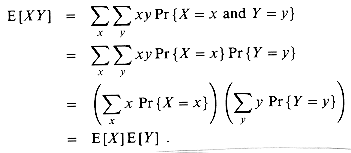
When two random variables X and Y are independent and each has a defined expectation,
In general, when n random variables X1, X2, . . . , Xn are mutually independent,
When a random variable X takes on values from the natural numbers N = {0,1, 2, . . .}, there is a nice formula for its expectation:
since each term Pr{X
The variance of a random variable X with mean E [X] is
The justification for the equalities E [E2 [X]] = E2 [X] and E [XE [X]] = E2 [X] is that E [X] is not a random variable but simply a real number, which means that equation (6.25) applies (with a = E[X]). Equation (6.29) can be rewritten to obtain an expression for the expectation of the square of a random variable:
The variance of a random variable X and the variance of aX are related:
When X and Y are independent random variables,
In general, if n random variables X1, X2, . . . , Xn are pairwise independent, then
The standard deviation of a random variable X is the positive square root of the variance of X. The standard deviation of a random variable X is sometimes denoted
6.3-1
Two ordinary, 6-sided dice are rolled. What is the expectation of the sum of the two values showing? What is the expectation of the maximum of the two values showing?
6.3-2
An array A[1 . . n] contains n distinct numbers that are randomly ordered, with each permutation of the n numbers being equally likely. What is the expectation of the index of the maximum element in the array? What is the expectation of the index of the minimum element in the array?
6.3-3
A carnival game consists of three dice in a cage. A player can bet a dollar on any of the numbers 1 through 6. The cage is shaken, and the payoff is as follows. If the player's number doesn't appear on any of the dice, he loses his dollar. Otherwise, if his number appears on exactly k of the three dice, for k = 1, 2, 3, he keeps his dollar and wins k more dollars. What is his expected gain from playing the carnival game once?
6.3-4
Let X and Y be independent random variables. Prove that f(X) and g(Y) are independent for any choice of functions f and g.
6.3-5
Let X be a nonnegative random variable, and suppose that E (X) is well defined. Prove Markov's inequality:
for all t > 0.
6.3-6
Let S be a sample space, and let X and X' be random variables such that X(s)
6.3-7
Which is larger: the expectation of the square of a random variable, or the square of its expectation?
6.3-8
Show that for any random variable X that takes on only the values 0 and 1, we have Var [X] = E [X] E [1 - X].
6.3-9
Prove that Var[aX] = a2Var[x] from the definition (6.29) of variance.
A coin flip is an instance of a Bernoulli trial, which is defined as an experiment with only two possible outcomes: success, which occurs with probability p, and failure, which occurs with probability q = 1 - p. When we speak of Bernoulli trials collectively, we mean that the trials are mutually independent and, unless we specifically say otherwise, that each has the same probability p for success. Two important distributions arise from Bernoulli trials: the geometric distribution and the binomial distribution.
Suppose we have a sequence of Bernoulli trials, each with a probability p of success and a probability q = 1 - p of failure. How many trials occur before we obtain a success? Let the random variable X be the number of trials needed to obtain a success. Then X has values in the range {1, 2, . . .}, and for k
since we have k - 1 failures before the one success. A probability distribution satisfying equation (6.33) is said to be a geometric distribution. Figure 6.1 illustrates such a distribution.
Assuming p < 1, the expectation of a geometric distribution can be calculated using identity (3.6):
Thus, on average, it takes 1/p trials before we obtain a success, an intuitive result. The variance, which can be calculated similarly, is
As an example, suppose we repeatedly roll two dice until we obtain either a seven or an eleven. Of the 36 possible outcomes, 6 yield a seven and 2 yield an eleven. Thus, the probability of success is p = 8/36 = 2/9, and we must roll 1/p = 9/2 = 4.5 times on average to obtain a seven or eleven.
How many successes occur during n Bernoulli trials, where a success occurs with probability p and a failure with probability q = 1 - p? Define the random variable X to be the number of successes in n trials. Then X has values in the range {0, 1, . . . , n}, and for k = 0, . . . , n,
since there are
Figure 6.2 illustrates a binomial distribution. The name "binomial" comes from the fact that (6.37) is the kth term of the expansion of (p + q)n. Consequently, since p + q = 1,
as is required by axiom 2 of the probability axioms.
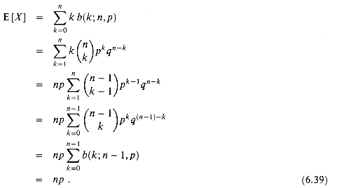
We can compute the expectation of a random variable having a binomial distribution from equations (6.14) and (6.38). Let X be a random variable that follows the binomial distribution b(k; n, p), and let q = 1 - p. By the definition of expectation, we have
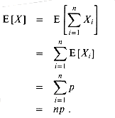
By using the linearity of expectation, we can obtain the same result with substantially less algebra. Let Xi be the random variable describing the number of successes in the ith trial. Then E[Xi] = p
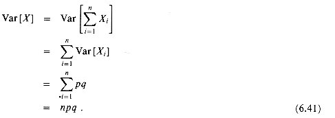
The same approach can be used to calculate the variance of the distribution. Using equation (6.29), we have
To compute the variance of X, we take advantage of the independence of the n trials; thus, by equation (6.31),
As can be seen from Figure 6.2, the binomial distribution b(k;n,p) increases as k runs from 0 to n until it reaches the mean np, and then it decreases. We can prove that the distribution always behaves in this manner by looking at the ratio of successive terms:
This ratio is greater than 1 precisely when (n + 1)p - k is positive. Consequently, b(k;n,p) > b(k - 1;n,p) for k < (n + 1)p (the distribution increases), and b(k;n,p) < b(k - 1;n,p) for k > (n + l)p (the distribution decreases). If k = (n + 1) p is an integer, then b(k;n,p) = b(k - 1;n,p), so the distribution has two maxima: at k = (n + l) p and at k - 1 = (n + 1)p - 1 = np - q. Otherwise, it attains a maximum at the unique integer k that lies in the range np - q < k < (n + 1)p.
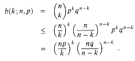
The following lemma provides an upper bound on the binomial distribution.
Lemma 6.1
Let n
Proof Using equation (6.10), we have
6.4-1
Verify axiom 2 of the probability axioms for the geometric distribution.
6.4-2
How many times on average must we flip 6 fair coins before we obtain 3 heads and 3 tails?
6.4-3
Show that b(k; n, p) = b(n - k; n, q), where q = 1 - p.
6.4-4
Show that value of the maximum of the binomial distribution b(k; n, p) is approximately
6.4-5
Show that the probability of no successes in n Bernoulli trials, each with probability p = 1/n, is approximately 1/e. Show that the probability of exactly one success is also approximately 1/e.
6.4-6
Professor Rosencrantz flips a fair coin n times, and so does Professor Guildenstern. Show that the probability that they get the same number of heads is
6.4-7
Show that for 0
where H(x) is the entropy function (6.13).
6.4-8
Consider n Bernoulli trials, where for i = 1,2, . . . ,n, the ith trial has probability pi of success, and let X be the random variable denoting the total number of successes. Let p
6.4-9
Let X be the random variable for the total number of successes in a set A of n Bernoulli trials, where the ith trial has a probability pi of success, and let X' be the random variable for the total number of successes in a second set A' of n Bernoulli trials, where the ith trial has a probability p'i
(Hint: Show how to obtain the Bernoulli trials in A' by an experiment involving the trials of A, and use the result of Exercise 6.3-6.)
The probability of having at least, or at most, k successes in n Bernoulli trials, each with probability p of success, is often of more interest than the probability of having exactly k successes. In this section, we investigate the tails of the binomial distribution: the two regions of the distribution b(k; n, p) that are far from the mean np. We shall prove several important bounds on (the sum of all terms in) a tail.
We first provide a bound on the right tail of the distribution b(k; n, p). Bounds on the left tail can be determined by inverting the roles of successes and failures.
Theorem 6.2
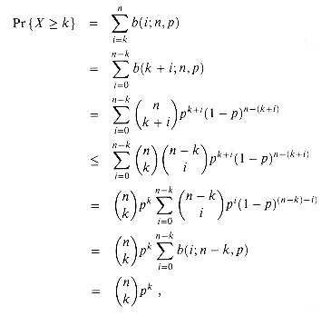
Consider a sequence of n Bernoulli trials, where success occurs with probability p. Let X be the random variable denoting the total number of successes. Then for 0
Proof We make use of the inequality (6.15)
We have
since
The following corollary restates the theorem for the left tail of the binomial distribution. In general, we shall leave it to the reader to adapt the bounds from one tail to the other.
Corollary 6.3
Consider a sequence of n Bernoulli trials, where success occurs with probability p. If X is the random variable denoting the total number of successes, then for 0
Our next bound focuses on the left tail of the binomial distribution. Far from the mean, the number of successes in the left tail diminishes exponentially, as the following theorem shows.
Theorem 6.4
Consider a sequence of n Bernoulli trials, where success occurs with probability p and failure with probability q = 1 - p. Let X be the random variable denoting the total number of successes. Then for 0 < k < np, the probability of fewer than k successes is
Proof We bound the series
If we let
it follows that
for 0 < i
for 0
When k
A bound on the right tail can be determined similarly.
Corollary 6.5
Consider a sequence of n Bernoulli trials, where success occurs with probability p. Let X be the random variable denoting the total number of successes. Then for np < k < n, the probability of more than k successes is
The next theorem considers n Bernoulli trials, each with a probability pi of success, for i = 1, 2, . . . , n. As the subsequent corollary shows, we can use the theorem to provide a bound on the right tail of the binomial distribution by setting pi = p for each trial.
Theorem 6.6
Consider a sequence of n Bernoulli trials, where in the ith trial, for i = 1, 2 , . . . , n, success occurs with probability pi and failure occurs with probability qi = 1 - pi. Let X be the random variable describing the total number of successes, and let
Proof Since for any
where
The bulk of the proof consists of bounding E[e
and
Substituting for X -
which follows from (6.27), since the mutual independence of the random variables Xi implies the mutual independence of the random variables e
where exp(x) denotes the exponential function: exp(x) = ex. (Inequality (6.44) follows from the inequalities
since
Choosing
When applied to Bernoulli trials in which each trial has the same probability of success, Theorem 6.6 yields the following corollary bounding the right tail of a binomial distribution.
Corollary 6.7
Consider a sequence of n Bernoulli trials, where in each trial success occurs with probability p and failure occurs with probability q = 1 - p. Then for
Proof For a binomial distribution, equation (6.39) implies that
6.5-1
Which is less likely: obtaining no heads when you flip a fair coin n times, or obtaining fewer than n heads when you flip the coin 4n times?
6.5-2
Show that
for all a > 0 and all k such that 0 < k < n.
6.5-3
Prove that if 0 < k < np, where 0 < p < 1 and q = 1 - p, then
6.5-4
Show that the conditions of Theorem 6.6 imply that
Similarly, show that the conditions of Corollary 6.7 imply that
6.5-5
Consider a sequence of n Bernoulli trials, where in the ith trial, for i = 1, 2, . . . , n, success occurs with probability pi and failure occurs with probability qi = 1 - pi. Let X be the random variable describing the total number of successes, and let
(Hint: Prove that pie
6.5-6
Show that choosing
This section uses three examples to illustrate probabilistic analysis. The first determines the probability that in a room of k people, some pair shares the same birthday. The second example examines the random tossing of balls into bins. The third investigates "streaks" of consecutive heads in coin flipping.
A good example to illustrate probabilistic reasoning is the classical birthday paradox. How many people must there be in a room before there is a good chance two of them were born on the same day of the year? The answer is surprisingly few. The paradox is that it is in fact far fewer than the number of days in the year, as we shall see.
To answer the question, we index the people in the room with the integers 1, 2, . . . , k, where k is the number of people in the room. We ignore the issue of leap years and assume that all years have n = 365 days. For i = 1, 2, . . . , k, let bi be the day of the year on which i's birthday falls, where 1
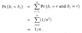
The probability that two people i and j have matching birthdays depends on whether the random selection of birthdays is independent. If birthdays are independent, then the probability that i's birthday and j's birthday both fall on day r is
Thus, the probability that they both fall on the same day is
More intuitively, once bi is chosen, the probability that bj is chosen the same is 1/n. Thus, the probability that i and j have the same birthday is the same as the probability that the birthday of one of them falls on a given day. Notice, however, that this coincidence depends on the assumption that the birthdays are independent.
We can analyze the probability of at least 2 out of k people having matching birthdays by looking at the complementary event. The probability that at least two of the birthdays match is 1 minus the probability that all the birthdays are different. The event that k people have distinct birthdays is
where Ai is the event that person (i + 1)'s birthday is different from person j's for all j
Since we can write Bk = Ak - 1
where we take Pr{B1} = 1 as an initial condition. In other words, the probability that b1, b2,...,bk are distinct birthdays is the probability that b1, b2, . . . , bk - 1, are distinct birthdays times the probability that bk
If b1, b2, . . . , bk - 1 are distinct, the conditional probability that bk
The inequality (2.7), 1 + x
when -k(k - l)/2n
We can use the linearity of expectation (equation (6.26)) to provide a simpler but approximate analysis of the birthday paradox. For each pair (i, j) of the k people in the room, let us define the random variable Xij, for 1
The probability that two people have matching birthdays is 1/n, and thus by the definition of expectation (6.23),
The expected number of pairs of individuals having the same birthday is, by equation (6.24), just the sum of the individual expectations of the pairs, which is
When k(k -1)
The first analysis determined the number of people required for the probability to exceed 1/2 that a matching pair of birthdays exists, and the second analysis determined the number such that the expected number of matching birthdays is 1. Although the numbers of people differ for the two situations, they are the same asymptotically:
Consider the process of randomly tossing identical balls into b bins, numbered 1, 2, . . . , b. The tosses are independent, and on each toss the ball is equally likely to end up in any bin. The probability that a tossed ball lands in any given bin is 1/b. Thus, the ball-tossing process is a sequence of Bernoulli trials with a probability 1/b of success, where success means that the ball falls in the given bin. A variety of interesting questions can be asked about the ball-tossing process.
How many balls fall in a given bin? The number of balls that fall in a given bin follows the binomial distribution b(k; n, 1/b). If n balls are tossed, the expected number of balls that fall in the given bin is n/b.
How many balls must one toss, on the average, until a given bin contains a ball? The number of tosses until the given bin receives a ball follows the geometric distribution with probability 1/b, and thus the expected number of tosses until success is 1/(1/b) = b.
How many balls must one toss until every bin contains at least one ball? Let us call a toss in which a ball falls into an empty bin a "hit." We want to know the average number n of tosses required to get b hits.
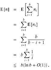
The hits can be used to partition the n tosses into stages. The ith stage consists of the tosses after the (i - 1)st hit until the ith hit. The first stage consists of the first toss, since we are guaranteed to have a hit when all bins are empty. For each toss during the ith stage, there are i -1 bins that contain balls and b - i + 1 empty bins. Thus, for all tosses in the ith stage, the probability of obtaining a hit is (b - i + 1)/b.
Let ni denote the number of tosses in the ith stage. Thus, the number of tosses required to get b hits is n =
By linearity of expectation,
The last line follows from the bound (3.5) on the harmonic series. It therefore takes approximately b ln b tosses before we can expect that every bin has a ball.
Suppose you flip a fair coin n times. What is the longest streak of consecutive heads that you expect to see? The answer is
We first prove that the expected length of the longest streak of heads is O(lg n). Let Aik be the event that a streak of heads of length at least k begins with the ith coin flip or, more precisely, the event that the k consecutive coin flips i, i+ 1, . . ., i+k - 1 yield only heads, where 1
and thus the probability that a streak of heads of length at least
since by Boole's inequality (6.22), the probability of a union of events is at most the sum of the probabilities of the individual events. (Note that Boole's inequality holds even for events such as these that are not independent.)
The probability is therefore at most 1/n that any streak has length at least 2
The chances that a streak of heads exceeds r
Thus, the probability is at most n/nr = 1/nr-1 that the longest streak is at least r
As an example, for n = 1000 coin flips, the probability of having a streak of at least 2
We now prove a complementary lower bound: the expected length of the longest streak of heads in n coin flips is
The probability that a streak of heads of length at least
For this argument, we used inequality (2.7), 1+ x
Thus, the probability that the longest streak exceeds
6.6-1
Suppose that balls are tossed into b bins. Each toss is independent, and each ball is equally likely to end up in any bin. What is the expected number of ball tosses before at least one of the bins contains two balls?
6.6-2
For the analysis of the birthday paradox, is it important that the birthdays be mutually independent, or is pairwise independence sufficient? Justify your answer.
6.6-3
How many people should be invited to a party in order to make it likely that there are three people with the same birthday?
6.6-4
What is the probability that a k-string over a set of size n is actually a k-permutation? How does this question relate to the birthday paradox?
6.6-5
Suppose that n balls are tossed into n bins, where each toss is independent and the ball is equally likely to end up in any bin. What is the expected number of empty bins? What is the expected number of bins with exactly one ball?
6.6-6
Sharpen the lower bound on streak length by showing that in n flips of a fair coin, the probability is less than 1/n that no streak longer than 1g n - 2 1g 1g n consecutive heads occurs.
6-1 Balls and bins
In this problem, we investigate the effect of various assumptions on the number of ways of placing n balls into b distinct bins.
a. Suppose that the n balls are distinct and that their order within a bin does not matter. Argue that the number of ways of placing the balls in the bins is bn.
b. Suppose that the balls are distinct and that the balls in each bin are ordered. Prove that the number of ways of placing the balls in the bins is (b + n - 1 )!/(b - 1)!. (Hint: Consider the number of ways of arranging n distinct balls and b - 1 indistinguishable sticks in a row.)
c. Suppose that the balls are identical, and hence their order within a bin does not matter. Show that the number of ways of placing the balls in the bins is
d. Suppose that the balls are identical and that no bin may contain more than one ball. Show that the number of ways of placing the balls is
e. Suppose that the balls are identical and that no bin may be left empty. Show that the number of ways of placing the balls is
6-2 Analysis of max program
The following program determines the maximum value in an unordered array A[1 . . n].
We want to determine the average number of times the assignment in line 5 is executed. Assume that all numbers in A are randomly drawn from the interval [0, 1].
a. If a number x is randomly chosen from a set of n distinct numbers, what is the probability that x is the largest number in the set?
b. When line 5 of the program is executed, what is the relationship between A[i] and A[j] for 1
c. For each i in the range 1
d. Let s1, s2, . . ., sn be n random variables, where si represents the number of times (0 or 1) that line 5 is executed during the ith iteration of the for loop. What is E[si]?
e. Let s = s1 + s2 +... + sn be the total number of times that line 5 is executed during some run of the program. Show that E[s] =
6-3 Hiring problem B| = |A| + |B|, which follows from equation (5.3). For example, each position on a car's license plate is a letter or a digit. The number of possibilities for each position is therefore 26 + 10 = 36, since there are 26 choices if it is a letter and 10 choices if it is a digit.
 B| = |A|
  |B|, which is simply equation (5.4). For example, if an ice-cream parlor offers 28 flavors of ice cream and 4 toppings, the number of possible sundaes with one scoop of ice cream and one topping is 28
  4 = 112.
Strings
000, 001, 010, 011, 100, 101, 110, 111 .
 n
n 

 n = nk as the number of k-strings.
Permutations
abc, acb, bac, bca, cab, cba .
ab, ac, ad, ba, bc, bd, ca, cb, cd, da, db, dc.

(6.1)
Combinations
ab, ac, ad, bc, bd, cd .

(6.2)
Binomial coefficients
 (read "n choose k") to denote the number of k-combinations of an n-set. From equation (6.2), we have
(6.3)

(6.4)

(6.5)

(6.6)
 binary n-strings containing exactly k 1's, since there are
  ways to choose k out of the n positions in which to place the 1's.
Binomial bounds
 k
k  n, we have the lower bound
(6.7)
 (k/e)k derived from Stirling's formula (2.12), we obtain the upper bounds
(6.8)
(6.9)
 k
k  n, we can use induction (see Exercise 6.1-12) to prove the bound
(6.10)
 n, where 0

 1, this bound can be rewritten as
(6.11)
(6.12)
H(
 ) = -
) = - lg
lg - (1 -
  ) lg (1 -
  )
)(6.13)
Exercises

(6.14)
 n.
n.
 k < n.
 k
k  n of the binomial coefficients
  with
with  at the top,
  and
and  on the next line, and so forth. Such a table of binomial coefficients is called Pascal's triangle.
 0 and 0
  k
k  n, the maximum value of
  is achieved when k =
  n/2
n/2 or k =
  n/2
n/2 .
. 0, j
0, j  0, k
0, k  0, and j + k
  n,
n,(6.15)
 n/2 to prove inequality (6.10), and use equation (6.4) to extend it to all k
  n.
n.(6.16)
 ), show that it achieves its maximum value at
  = 1/2. What is H (1/2)?
6.2 Probability
S = {HH, HT, TH, TT} . is called the null event. We say that two events A and B are mutually exclusive if
  . We sometimes treat an elementary event s
  S as the event {s}. By definition, all elementary events are mutually exclusive.
Axioms of probability
 0 for any event A.
 B} = Pr {A} + Pr {B} for any two mutually exclusive events A and B. More generally, for any (finite or countably infinite) sequence of events A1, A2, . . . that are pairwise mutually exclusive,
 has probability
  . If A
  B, then Pr{A}
  Pr{B}. Using
  to denote the event S - A (the complement of A), we have
  . For any two events A and B,
PR{A  B} = Pr{A} + Pr{B} - Pr{A
  B}
B}(6.17)
 Pr{A} + Pr{B} .
(6.18)
Pr{HH, HT, TH} = Pr{HH} + Pr{HT} + Pr{TH}= 3/4.
Discrete probability distributions

 S has probability
Pr{s} = 1/ S
S ,
,A = {exactly k heads and exactly n - k tails occur} , since there are
  strings of length n over {H, T} that contain exactly k H'S. The probability of event A is thus
  .
.Continuous uniform probability distribution
 c
c  d
d  b, the continuous uniform probability distribution defines the probability of the event [c, d] to be
 (c, d)
  [d, d], axiom 3 gives us Pr{[c, d]} = Pr{(c, d)}. Generally, the set of events for the continuous uniform probability distribution is any subset of [a, b] that can be obtained by a finite or countable union of open and closed intervals.
Conditional probability and independence

(6.19)
 0. (We read "Pr{A
  B}" as "the probability of A given B.") Intuitively, since we are given that event B occurs, the event that A also occurs is A
  B. That is, A
  B is the set of outcomes in which both A and B occur. Since the outcome is one of the elementary events in B, we normalize the probabilities of all the elementary events in B by dividing them by Pr{B}, so that they sum to 1. The conditional probability of A given B is, therefore, the ratio of the probability of event A
  B to the probability of event B. In the example above, A is the event that both coins are heads, and B is the event that at least one coin is a head. Thus, Pr{A
  B} = (1/4)/(3/4) = 1/3.
Pr{A  B} = Pr{A}Pr{B},
 0, to the condition
Pr{A B} = Pr{A}.
 (1/2)(1/2). Consequently, the event that one comes up heads and the event that the other comes up heads are not independent.
Pr{Ai  Aj} = Pr{Ai} Pr{Aj}
 i < j
i < j  n. We say that they are (mutually) independent if every k-subset Ai1,Ai2,...,Aik of the collection, where 2
  k
k  n and 1
  i1 < i2 <

 < ik
< ik  n, satisfies
Pr{Ai1  Ai2
Ai2 


 Aik} = Pr{Ai1}Pr{Ai2}

 Pr{Aik}.
 Pr{A1} = 1/2 , Pr{A2} = 1/2 , Pr{A3} = 1/2 , Pr{A1  A2} = 1/4 ,
 Pr{A1  A3} = 1/4 ,
 Pr{A2  A3} = 1/4 ,
Pr{A1  A2
A2  A3} = 0.
 i < j
i < j  3, we have Pr{Ai
  Aj} = Pr{Ai}Pr{Aj} = 1/4, the events A1, A2, and A3 are pairwise independent. The events are not mutually independent, however, because Pr{A1
  A2
A2  A3} = 0 and Pr{A1} Pr{A2} Pr{A3} = 1/8
  0.
0.Bayes's theorem
Pr{A  B} = Pr{B}Pr{A|B}
(6.20)
= Pr{A}Pr{B|A}.
(6.21)
 and B
and B  A and
A and  are mutually exclusive events,

 hence,
Exercises
Pr{A1  A2
A2 


 }
}  Pr{A1} + Pr{A2}+

 .
.(6.22)

Pr{A1  A2
A2 


 An} = Pr{A1}
  Pr{A2 | A1}
  Pr{A3 | A1
  A2}
A2}


Pr{An | A1  A2
A2 


 An-1}.
Pr{A  B | C} = Pr{A | C}
  Pr{B | C} .
6.3 Discrete random variables
 S : X (s) = x}; thus,
f(x) = Pr{X = x} 0 and
0 and  x Pr{X = x} = 1.
 S is equally likely: Pr {s} = 1/36. Define the random variable X to be the maximum of the two values showing on the dice. We have Pr {X = 3} = 5/36, since X assigns a value of 3 to 5 of the 36 possible elementary events, namely, (1, 3), (2, 3), (3, 3), (3, 2), and (3, 1).
f(x,y) = Pr{X = x and Y = y}


Expected value of a random variable

(6.23)
 x or, when the random variable is apparent from context, simply by
  .
.E[X] = 6
 Pr{2 H'S} + 1
  Pr{1 H, 1 T} - 4
  Pr{2 T'S}
= 6(1/4)+ 1(1/2) - 4(1/4)
= 1 .
E[X + Y] = E[X] + E[Y] ,
(6.24)

E[aX] = aE[X] .
(6.25)
E[aX + Y] = aE[X] + E[Y] .
(6.26)
E[X1X2


 Xn] = E[X1]E[X2]

 E[Xn] .
(6.27)

(6.28)
 i} is added in i times and subtracted out i - 1 times (except Pr{X
  0}, which is added in 0 times and not subtracted out at all).
Variance and standard deviation
Var[X] = E[(X - E[X])2]
= E[X2 - 2XE[X] + E2[X]]
= E[X2] - 2E[XE[X]] + E2[X]
= E[X2] - 2E2[X] + E2[X]
= E[X2] - E2[X].
(6.29)
E[X2] = Var[X] + E2[X].
(6.30)
Var[aX] = a2Var[X].
Var[X + Y] = Var[X] + Var[Y].

(6.31)
 x or simply
  when the random variable X is understood from context. With this notation, the variance of X is denoted
  2.
2.Exercises
Pr{X  t}
t}  E[X]/t
 (6.32)
 X'(s) for all s
  S. Prove that for any real constant t,
Pr{X  t}
t}  Pr{X'
Pr{X'  t} .
t} .6.4 The geometric and binomial distributions
The geometric distribution
 1,
1,Pr{X = k} = qk-1p ,(6.33)
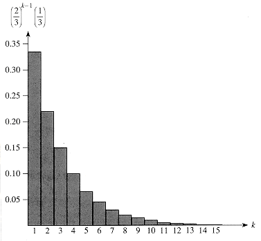
Figure 6.1 A geometric distribution with probability p = 1/3 of success and a probability q = 1 - p of failure. The expectation of the distribution is 1/p = 3.

(6.34.)
Var[X] = q/p2 .
(6.35)
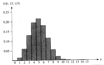
Figure 6.2 The binomial distribution b(k; 15, 1/3) resulting from n = 15 Bernoulli trials, each with probability p = 1/3 of success. The expectation of the distribution is np = 5.
The binomial distribution

(6.36)
 ways to pick which k of the n trials are successes, and the probability that each occurs is pkqn-k. A probability distribution satisfying equation (6.36) is said to be a binomial distribution. For convenience, we define the family of binomial distributions using the notation
(6.37)

(6.38)
(6.39)
 1+ q
1+ q  0 = p, and by linearity of expectation (6.26), the expected number of successes for n trials is
 . Since Xi only takes on the values 0 and 1, we have
  , and hence
Var[Xi] = p - p2 = pq .
(6.40)
(6.41)

(6.42)
 0, let 0 < p < 1, let q = 1 - p, and let 0
  k
k  n. Then
Exercises
 where q = 1 - p.
 . (Hint: For Professor Rosencrantz, call a head a success; for Professor Guildenstern, call a tail a success.) Use your argument to verify the identity
 k
k  n,
n,b(k;n, 1/2)
 2nH(k/n)-n,
 pi for all i = 1, 2, . . . , n. Prove that for 1
  k
k  n,
n,
 pi of success. Prove that for 0
  k
k  n,
n,Pr{X'  k}
k}  Pr{X
Pr{X  k} .
k} .* 6.5 The tails of the binomial distribution
 k
k  n, the probability of at least k successes is

 by equation (6.38).
  k
k  n, the probability of at most k successes is

 by a geometric series using the technique from Section 3.2, page 47. For i = 1, 2, . . . , k, we have from equation (6.42),
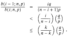

b(i - 1;n,p) < x b(i;n,p)
 k. Iterating, we obtain
b(i;n,p) < xk-i b(k;n,p)
 i < k, and hence
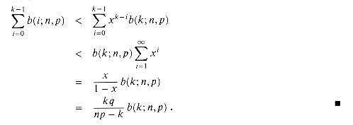
 np/2, we have kq/(np - k)
  1, which means that b(k; n, p) bounds the sum of all terms smaller than k. As an example, suppose we flip n fair coins. Using p = 1/2 and k = n/4, Theorem 6.4 tells us that the probability of obtaining fewer than n/4 heads is less than the probability of obtaining exactly n/4 heads. Furthermore, for any r
  4, the probability of obtaining fewer than n/r heads is less than that of obtaining exactly n/r heads. Theorem 6.4 can also be quite useful in conjunction with upper bounds on the binomial distribution, such as Lemma 6.1.
 = E[X]. Then for r >
  ,
,
 > 0, the function e
 x is strictly increasing in x,
Pr{X - 
 r} = Pr{e
 (X-
(X- )
)  e
e r} ,
r} , will be determined later. Using Markov's inequality (6.32), we obtain
Pr{X - 
 r}
r}  E[e
E[e (X-
(X- )]e-
)]e- r .
r .(6.43)
 (X-
(X- )] and substituting a suitable value for
  in inequality (6.43). First, we evaluate E[e
 (X-
(X- )]. For i = 1, 2, . . . , n, let Xi be the random variable that is 1 if the ith Bernoulli trial is a success and 0 if it is a failure. Thus,

 , we obtain
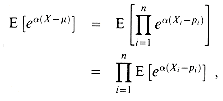
 (Xi-pi) (see Exercise 6.3-4). By the definition of expectation,
E [e
 (Xi-pi)] = e
 (1-pi) pi + e
 (0-pi) qi
= pie
 qi + qie-
 pi
pi pie
pie + 1
+ 1 ex(pie
 ) ,
) ,(6.44)
 > 0, q
  1, e
1, e q
q e
e , and e-
 p
p  1, and the last line follows from inequality (2.7)). Consequently,
 . Hence, from inequality (6.43), it follows that
Pr{X - 
 r}
r}  exp(
exp( e
e -
-  r) .
r) .(6.45)
 = 1n(r/
 ) (see Exercise 6.5-6), we obtain

 = E [X] = np.
 Exercises


 = E [X]. Show that for r
  0,
0,Pr{X -  ]
]  r}
r}  e-r2/2n.
 qi + qie-
 pi
pi  e-
e- 2/2. Then follow the outline of the proof of Theorem 6.6, using this inequality in place of inequality (6.44).)
 = 1n(r/
 ) minimizes the right-hand side of inequality (6.45).
6.6 Probabilistic analysis
6.6.1 The birthday paradox
 bi
bi  n. We also assume that birthdays are uniformly distributed across the n days of the year, so that Pr{bi = r} = 1/n for i = 1, 2, . . . , k and r = 1, 2, . . . , n.
Pr{bi = r and bj = r} = Pr{bi = r}Pr {bj = r}= 1/n2 .

 i, that is,
Ai = {bi +1  bj: j = 1, 2 . . . , i}.
 Bk - 1, we obtain from equation (6.20) the recurrence
Pr{Bk} = Pr{Bk - 1}Pr{Ak - 1  Bk - 1} ,
(6.46)
 bi for i = 1, 2, . . . , k - 1, given that b1,b2,...,bk - 1 are distinct.
 bi for i = 1, 2, . . . , k - 1 is (n - k + 1)/n, since out of the n days, there are n - (k - 1) that are not taken. By iterating the recurrence (6.46), we obtain
 ex, gives us
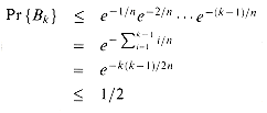
 ln(1/2). The probability that all k birthdays are distinct is at most 1/2 when k(k - 1)
  2n ln 2 or, solving the quadratic equation, when
  . For n = 365, we must have k
  23. Thus, if at least 23 people are in a room, the probability is at least 1/2 that at least two people have the same birthday. On Mars, a year is 669 Martian days long; it therefore takes 31 Martians to get the same effect.
Another method of analysis
 i
i  j
j  k, by
k, by
E[Xij] = 1
 (1/n) + 0
  (1 - 1/n)
= 1/n.

 2n, therefore, the expected number of pairs of birthdays is at least 1. Thus, if we have at least
  individuals in a room, we can expect at least two to have the same birthday. For n = 365, if k = 28, the expected number of pairs with the same birthday is (28
 27)/(2
 365)
365)  1.0356. Thus, with at least 28 people, we expect to find at least one matching pair of birthdays. On Mars, where a year is 669 Martian days long, we need at least 38 Martians.
 .
.6.6.2 Balls and bins
 . Each random variable ni has a geometric distribution with probability of success (b - i + 1)/b, and therefore
6.6.3 Streaks
 (lg n), as the following analysis shows.
 k
k  n and 1
  i
i  n - k + 1. For any given event Aik, the probability that all k flips are heads has a geometric distribution with p = q = 1/2:
Pr {Aik} = 1/2k .(6.47)
For k = 2
 lg n
lg n ,
,Pr{Ai,2 1g n
1g n } = 1/2 2
 1g n
1g n
 1/2 2 1g n
= 1/n2,
 2 1g n
 begins in position i is quite small, especially considering that there are at most n positions (actually n - 2
 1g n
1g n  + 1 ) where the streak can begin. The probability that a streak of heads of length at least
  2 1g n
 begins anywhere is therefore
 1g n
1g n ; hence, the probability is at least 1 - 1/n that the longest streak has length less than 2
  1g n
1g n . Since every streak has length at most n, the expected length of the longest streak is bounded above by
(2
 lg n
lg n )(1 - 1/n) + n(1/n) = O(lg n).
 1g n
1g n flips diminish quickly with r. For r
  1, the probability that a streak of r
  1g n
1g n heads starts in position i is
Pr{Ai,r 1g n
1g n } = 1/2r
 lg n
lg n
 1/nr.
1/nr. 1g n
1g n , or equivalently, the probability is at least 1- 1/nr-1 that the longest streak has length less than r
  1g n
1g n  .
. 1g n
1g n = 20 heads is at most 1/n = 1/1000. The chances of having a streak longer than 3
  1g n
1g n = 30 heads is at most 1/n2 = 1/1,000,000.
 (1g n). To prove this bound, we look for streaks of length
  1g n
1g n /2. From equation (6.47), we have
 1g n
1g n /2 does not begin in position i is therefore at most
  . We can partition the n coin flips into at least
  2n/
2n/  1g n
1g n
 groups of
  1g n
1g n /2 consecutive coin flips. Since these groups are formed from mutually exclusive, independent coin flips, the probability that every one of these groups fails to be a streak of length
  1g n
1g n /2 is
/2 is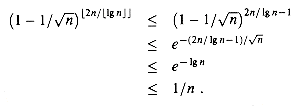
 ex, and the fact, which you might want to verify, that (2n/1g n - 1) /
 1g n for n
  2. (For n = 1, the probability that every group fails to be a streak is trivially at most 1/n = 1.)
 1g n
1g n /2 is at least 1- 1/n. Since the longest streak has length at least 0, the expected length of the longest streak is at least
(
 1g n
1g n /2)(1 - 1/n) + 0
 (1/n) =
  (1g n).
Exercises
Problems
 . (Hint: Of the arrangements in part (b), how many are repeated if the balls are made identical?)
 .
. .
.1 max
 -
-
2 for i
 1 to n
3 do
 Compare A[i] to max.
4 if A[i] > max
5 then max
 A[i]
A[i] j
j  i?
i? i
i  n, what is the probability that line 5 is executed?
 (lg n).


