Unlock(door)
is a neat solution to a problem--if you have a key (that is, if the procedure Unlock can be rendered in a practical way). Pseudocode is used in the pages that follow, but we keep in mind that algorithms are to be translated into a working language before use, with a structured language such as Pascal, ADA, or Modula-2. Clean, logical structures are easier to translate into these languages than into others, but each language has its own foibles because each is itself the result of choices.
The conversion of a pseudocode description of an algorithm into a working language is a learning experience that focuses on the logic involved and distinguishes that logic from language features. A program or procedure given in executable form can be applied blindly and without understanding. Pseudocode requires some attention but no major effort to translate. At the same time, translating an algorithm into code is much quicker and easier than deriving the algorithm itself and thus increases the amount of material that can be applied in a limited time.
The meaning of each of the pseudocode structures used in this book is explained in the next section.
Note: Part II of this book, "Expansions and Applications," includes working programs realized in Pascal. They implement some of the procedures presented in pseudocode in the main part of the text.
1.2 The Pseudocode Language SUE
If it weren't for the powerful effects of data structures and of other ideas, commands given to computers could be comfortably limited to six basic operations:
1. Copy data from one memory cell to another.
2. Perform arithmetic and logical operations.
3. Input data: place data from the outside world into memory.
4. Output data: retrieve data from memory and send it to the outside world.
5. Branch unconditionally to some command.
6. Branch on the truth of a condition to some command.
These commands are communicated to a computer from a translator (usually a compiler or assembler). The translator derives the commands from statements in the language being translated. Because such statements need to be explicit and unambiguous, they involve rules of syntax and conventions that are not really required to describe the logic of a program. Algorithms, which communicate program logic to people, can be reduced to simpler and more universal statements than current working languages allow.
The logical structures that follow are universal in the sense that the ideas involved can be implemented in any language. The language SUE is designed to focus attention on these logical structures, to be flexible, and to be expandable as required. All of the algorithms in this book are described in SUE.
Note: The name SUE has been used for other languages, but it is difficult to avoid all short mnemonics; SUE is used here only as a useful abbreviation.
The essential constructs of SUE are
Read and Write are intended to be more general than they are in most working languages. Variables may be of any structural type in SUE. The format of the output of an array, record, or other variable type is provided during the translation of SUE into a working language:
For example
will, when A = 2, B = 3, and C = 1, display 2. By contrast, if the else were taken to be the alternate condition for the first if, there would be no output from this segment. Astute indention may resolve an else for the human reader, but it will not do so for a computer, and so endif terminates all if statements in the text.
Another kind of selection statement is case, which may appear in two forms:
General case structures sometimes must be resolved in terms of nested if . . . then . . . else statements in a program.
Loop structures may be classified by the location of the test for exit from the loop: at the top, at the bottom, or in the middle. They all must determine the beginning and the end of the loop; that is, what is included and what is not, as well as the exit-test position. The three essential loop forms in SUE are:
Note: Not all structured languages (notably standard Pascal) provide for exit. An exit can be made from any loop by declaring a label and using a GOTO (an unconditional branch).
An example of a GOTO in Pascal is
A common mode of looping is the use of a control variable as a counter to keep track of the passes through a loop. This may be done in SUE with:
The for loop is equivalent to the following, with one disclaimer stated below:
The disclaimer is that--in some languages and on some machines--compiler programs apply sophisticated (increment-and-branch) instructions in the translation of the for loop construct. The exact translation is determined by the writer(s) of the compiler and influenced by the properties of the hardware, not by definition of the language alone. Although the for loop is usually implemented in programming languages as a while, this is not always the case. For example, the FOR . . . NEXT loop in at least one heavily used BASIC translator is essentially a repeat . . . until structure, as is the analogous FORTRAN DO loop. In SUE, a for is a specific form of while, and the value of v immediately upon completion of the loop is unknown.
Computing languages differ in the way they pass information between programs or between parts of one program. SUE simplifies the description of information- sharing as much as possible, while remaining consistent with the modularization of programs in structured languages.
A procedure in SUE is a segment of code that is independent in the sense that it can be invoked conveniently, it does a specified task, and it then returns control to the point immediately following its invocation. A program is itself a procedure that may invoke functions or other procedures, called subprograms. A list of parameters that provide information to or return information from a procedure may be included in the invocation and the definition. Variables not listed are considered to be global (defined and available outside of the procedure). As an example:
The variable Sum is global to AddAbs, but v is local. This means that the identifier v is redefined within AddAbs, and its relationship to x and y is determined at the time of individual invocations. Identifier v is a parameter that is related to x the first time, and to y in the second call.
The formal parameter v can be related to actual parameters x and y in two major ways:
1. Treat x (or y) as an expression. Its value is stored locally in v. No other information about the source is available to Abs. In this case, v is called a value parameter.
2. Treat x (or y) as an address. The address is stored in v, which becomes a pointer. Whenever an assignment is made in Abs to v, the assignment is actually to the (actual) parameter x. In this case, v is called a variable parameter.
The passing of parameters to subprograms is a major topic in programming languages, and no attempt to resolve or restrict it is made in SUE. A parameter in SUE may be of either type, but it is generally left unspecified. The choice may be important during implementation of an algorithm in a specific language. The best guide to making this choice is an understanding of the algorithm.
A function in SUE is a procedure that returns a single value. A function, therefore, may be invoked by using it anywhere that a variable can be used. The result that it calculates becomes the value of the function name. For example:
The essential distinction between Abs and AddAbs is that the identifier Abs is assigned a value in its definition and can be used to retrieve that value, but the identifier AddAbs has no assigned value--it is the name of a subprogram that performs a task.
A valuable tool for presenting the logic of some algorithms (and for implementing them when it is available) is return. A return may be used to exit immediately from a subprogram at any point. If the subprogram is a function, return v indicates that v is to be returned as the functional value. When it is not available as a language feature, return is implemented much like exit.
The correspondence between Pascal, for example, and SUE can be quite close:
Note: Simplifications applied in this book are the use of global variables and of multiple exits (from loops) and multiple returns (from subprograms). It is only their thoughtful use that is being endorsed here, and they may be routinely removed when algorithms are translated into a working language.
For the sake of completeness, records and pointers are reviewed in this section.
In a gradebook program, a name and a score may be kept in separate arrays (because they are of different types) and tied together logically by giving them the same index. An alternate storage structure for the names and scores is a record, perhaps declared by:
A record, as it is used here, is a data structure in its own right, available in many languages. As a structure, however, it differs from the array structure in only two ways:
1. The cells of a record do not need to contain data of identical type.
2. The identifier of a cell (called a field in a record) is not an index, but a name. For a variable Good of type Result, Good.Name identifies the field of type STRING and Good.Score identifies the field of type INTEGER.
Some data structures are formed from records called nodes that are linked together in the sense that a node contains the address of one or more other nodes. Such addresses are made available as variables so they can be altered. A variable that contains the address of data, rather than the value of data in question, is called a pointer variable.
In a simple structure, nodes may contain single values (of some type). Each node also contains an address value, called a link,and so it can be declared to be:
For a variable xNode of type Nodule, xNode.Value is the name of the field of type REAL, and xNode.Link is the name of the field of type
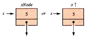
Suppose that xNode is a record of type Nodule. A pointer to a record like xNode assumes the role of a node identifier, simply because a pointer, like an identifier, is a locator. (Both technically determine more information than simply an address, but it is the same information as that provided by languages that allow pointer variables.) If x is a pointer to xNode, then x
If xNode is of type Nodule, then x is of type
without an assumed initialization of p
Comparisons of algorithms are made on the basis of the management of resources, and one crucial resource is execution time. It is generally not necessary to determine exact execution times, which may be data-dependent or machine-dependent anyway and which can be seriously misleading in interactive systems. There is an important difference, however, between an algorithm that takes a minute or so to run and one that takes an hour.
The difference in execution times between two approaches to solving a problem may be small for small data sets; for large data sets, by contrast, the execution times of one approach may grow very differently from those of the other. For algorithms that are to be used many times, any difference can be significant, but generally an analysis of execution time concentrates on how it grows with the increasing size of data sets.
The growth of execution time as a function of the size of the problem data provides a basis for comparing ways of solving the problem.
A simple approach that is frequently adequate for our purposes can be applied to the following program segment:
An analysis may begin by assuming that [statement k] takes one unit of time for k = 1,2,3. Then this segment requires one unit of time for [statement 1] followed by two units of time for each pass through the for loop. Therefore, the execution time is
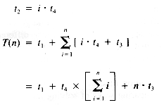
This can be easily generalized by assuming that [statement i] requires ti units of time:
This equation remains true even if [statement 2] is itself a loop that always requires the same amount of time to execute. For example, if [statement 2] is
Complications arise, however, if the execution of [statement 2] depends upon i:
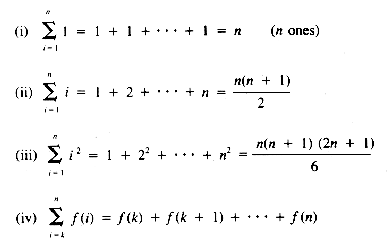
At this point, we need to document some of the properties of summations, because loop execution times are a sum of the times required for each pass through them.
where k < n and f is any function of i
where a and b are not functions of i
From equation ii, then, the value of T(n) is:
If it may be assumed that t1 = t3 = t4 = 1, then:
a quadratic function on n.
As a more specific example, consider:
EP1.1 Input n numbers, and list those that follow the occurrence of the minimal entry value.
One solution is:
In order to make a detailed analysis of the execution time of TrailMin, it would be necessary to assume some relative execution times of the Read, Write, if, and assignment statements and to perhaps consider the test-for-exit overhead implicit in the for statement. A first approximation ignores these differences and concentrates on the number of times that statements are executed. This provides a basis for an overview of the behavior of an algorithm.
With the simplifying assumption that each statement requires one unit of time, the timing function for TrailMin is:
Clearly, though, Mindex may be a function of n itself. In section 1.3.2 it is shown that Mindex can be expected to have the middle value (n + 1)/2, and so T(n) may be taken to be (5n/2) - 1/2 as a reasonable approximation. If the point of the analysis is the growth of T(n) as n increases, then it is enough to have found that T(n) is of the form: a
The growth behavior of an algorithm is quite often taken to be the salient fact revealed by timing analysis, and it will be explored further in the next section. Growth behavior provides a way to choose between algorithms that are to be applied to large data sets.
Another way to characterize Mindex as a function of n arises from the recognition that the execution time of Mindex is partly determined by the distribution of values in the sequence of entries. Random variation plays a role in the behavior of algorithms, and thus statistics should play a role both in the comparison of algorithms and in the study of the data structures on which they are founded. (See section 1.3.2.)
The analysis of algorithms includes the study of the worst-case data set of a given size, the (statistical) average case, and the limits imposed by the problem itself. In some cases, results of importance are derived experimentally. In this text, the intent is in a rough but convenient measure that is fairly easy to recognize for common algorithms. That measure is the order of growth.
1.3.2 The Variability of Data (optional)
Not all timing functions are linear in the size of the data set being processed. Common timing functions include quadratics and other polynomials, logarithms (a base of 2 is used in such studies), exponential functions, and others. These functions grow with n at dramatically different rates, as Table 1.1 reveals.
Suppose that procedure A and procedure B are both solutions to the same problem, and the timing functions for A and B are:
Suppose further that a time unit is 1 microsecond (10-6 second). Then whenever n = 1024, TA(n) is about 0.01 second, and TB(n) is about 1 second. However, for n = 65536, TA(n) is about 1 second, and TB(n) is roughly 1 hour and 12 minutes. If these procedures need to be used several times to accomplish some task, then procedure B becomes impractical for large data sets. A third procedure with T(n) = 2n would require 2.81 X 10¹⁴ years to deal with just 48 data values, and that is about 20,000 times as long as the age of the universe! Clearly, algorithms with execution times that grow exponentially are to be avoided for large data sets. Unfortunately, for many very important problems, all known solutions grow exponentially. Research in the theory of algorithms is being actively pursued to study that kind of behavior and other problems.
When it is desirable to determine the growth rate of a function, it is useful to eliminate as many extraneous details as possible. As n grows large, any linear function TL(n) = a
Comparison of growth rates is made explicit by the following:
DEFINITION: f(n) = O(g(n)) iff (if and only if) there exist constants c and m such that |f(n)|
The term O(g(n)) is read "big Oh of g of n." The statement f(n) = O(g(n)) says, in effect, that g(n) grows at least as fast as f(n). An example of its formal use is a
for all n > 1.
We need only to extract the kernel of this approach:
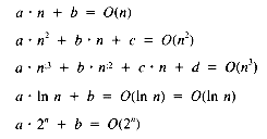
The most useful orders and their relative growth rates are:
Any polynomial has an order less than the order of an exponential function. The fastest growth rate dominates, and so, for example
for any polynomial P(n).
Fortunately, the order of an algorithm can often be found without going through a detailed analysis. Consider:
The order is clearly O(n) as long as statements 1, 2, and 3 may be assigned unit time. If they call other procedures, however, then it may be necessary to use the analysis techniques at the beginning of section 1.3.
There are some important points to note about the analysis of algorithms:
If large data sets are to be handled by a procedure, then the order of its timing function is of great concern. It may be possible to recognize the order without a detailed analysis, as we will often do, and some approaches can be dismissed on that basis.
It is possible to place too much emphasis on the order of T. Many procedures are applied exclusively to relatively small data sets. If so, concern with O(T(n)) may obscure an important difference in the execution times of two algorithms.
The variability of data sets can profoundly affect the behavior of an algorithm. Much of statistics can be brought to bear on the study of computing processes in situations where it is useful to do so.
Some well-known algorithms have defied analysis, and others arise in practice that are not cost-effective to analyze in detail, even if one is prepared and able to make the analysis. It is possible, and sometimes profitable, to study procedures experimentally by varying data sets and observing the reaction of the procedures to the changes.
Exercise E1.1 and problem P1.1 are appropriate at this time.
When TrailMin (see section 1.3) is examined in terms of the order of growth, it is evident that T(n) = O(n), no matter what value Mindex has. For a more detailed analysis, it is necessary to study the variations of Mindex. The statistical tool that is required is a statistical average, the expected value. If a variable, x, can take on values with probability P[x], then the expected value is:
The possible values of Mindex are 1, 2, . . ., n. If they are all equally likely, then their probabilities are all equal to 1/n. Hence:
It may be known, however, that Mindex values tend to occur late in the sequence of entries. Suppose, for example, that the probability is q when Mindex = 1, 2q when Mindex = 2, and in general, kq when Mindex = k, for k = 1, 2, . . ., n. One of these has to be the value, so the probabilities sum to 1:
And so
whence:
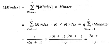
Now the expected value of Mindex is:
With this result, using E[Mindex] to represent Mindex:
There are many ways to sort data, and most of them have appropriate applications. The three ways that will be explored here are not suitable for large data sets, but they are relatively easy to understand and may be familiar already. The essential problem to be solved is:
EP1.2 Input n numbers, sort them, and then display them in nonincreasing order.
A whimsical solution, which is also the solemn solution of top-down programmers, is:
The procedures Ingress and OutHaul are quickly analyzed:
Systems analysts might leave the grubby details of Sort to a (lower-paid) junior programmer. We would be derelict in our duty if we did this because Sort is the heart of procedure InOut. Thus, the decision about which sorting technique should be used is a major one. The splitting of InOut into three procedures allows us to concentrate on the kernel of the problem without distractions. The difficulties are put off and isolated, in this case by dealing with input and output external to Sort.
One sorting technique begins by searching the entries for a maximal value and exchanging it with e[1]. The maximal value is then in e[1]. A repeat finds a maximal value of the other n - 1 entries and exchanges it with e[2]. Exchanges continue until e[n - 1] is in its proper place. When the first n - 1 values are arranged in nonincreasing order in this way, they are all in their proper places. Figure 1.1 is a series of snapshots of the process.
This process can be implemented by using the variable Target as the index of the position into which a maximal value is being exchanged. Then, for each value of Target from 1 to n - 1, a search is made for the maximal value of e[i], for all i
If the time required to carry out the hunt is t, and a unit time is required for assignment statements, then the timing function of SelectionSort is:
Hunt must be developed in order to resolve this further:
We see that Hunt, in fact, is a function of Target, and should properly be denoted by Hunt(Target). The timing function for Hunt, if the statistical behavior of the if statement is ignored, is:
If it is necessary to know the statistical behavior of the if, then the analysis becomes more complex. One must decide on probabilities for the condition of the if to be TRUE on any given pass through the for loop. Such a detailed analysis is generally uncalled for, because the intent is often to get a reasonable estimate of the behavior of SelectionSort to compare it with other sorting algorithms. Of course, if the distribution of data values is known, and the growth behaviors of the algorithms are similar, then it may be worth the effort.
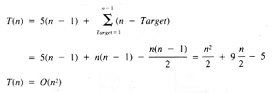
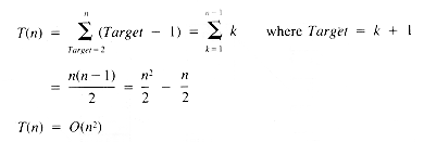
With the t that was calculated above:
The O(n2) result is no surprise, since it is often produced by a loop within a loop. One would be suspicious of any other result.
Exercise E1.2 is appropriate at this point.
Procedure SelectionSort moves the maximal value to the top of e in a direct way; smaller values eventually move toward the bottom. Another way to produce the same effect is to slide the smallest value to the bottom of e, as it is encountered on the first pass, then the second-smallest to the next-to-last position on the second pass, and so on. Because the smallest item cannot be recognized until a pass is complete, the smallest item so far slides downward during each pass. (This general technique is called a bubble sort here and in other places, although some programmers reserve that term for particular variations.) Large values slowly rise like a bubble in liquid, one position per pass.
Snapshots of the process that follow assume that the data in an array are originally in this order:
BubbleSort proceeds by rearranging the data on the first pass as shown in Figure 1.2.
The final result of the second, third, fourth, and fifth passes is shown in Figure 1.3.
One version of the process is:
Clearly,
for BubbleSort, where t is the timing function for Slide. "Sliding" really means "exchanging as we go," so Slide becomes:
With the assumption that the if statement requires one unit of time, the timing function for Slide is
whence For Slide:
The surprise here is how similar the timing is for SelectionSort and BubbleSort, rather than how different. There may be a considerable difference, of course, if they are used many times on small data sets in some process. Differences in speed between algorithms with similar timing functions can be very data dependent and even reversed by some sets of data. One effect of chance is the number of exchanges actually made in Slide. An experimental comparison of algorithms may be in order if a critical choice is to be made between them.
A number of modifications can be made to BubbleSort, such as:
Clear a flag variable just before entering Slide and reset it if an exchange is made. If the flag remains cleared, then the entries are already in order, and so successive passes may be aborted.
Make one pass down, sliding small values; and make the next one up, sliding large values. The rationale for this is that when sliding down, a small value may move a long way, but a large value can bubble only one step up. There is then a choice between splitting Slide into Slideup and Slidedown or generalizing it to handle both directions.
Some modifications of BubbleSort are more efficient for some data sets, but not necessarily for all.
Exercise E1.3 is appropriate at this point.
Neither SelectionSort nor BubbleSort seems to be natural to card players. Most people sort cards as they are received from the dealer, one at a time. The first card is simply picked up. The second card is placed on the correct side of the first. The third goes on the outside of the first two or between them, and so on. The crux of this process is that the items input so far are always in order; thus, it is easy to search through them for the proper position of the next one. Rather than combine Ingress with Sort in procedure InOut, we will use the same process in situ: e[1] is the first value, e[2] is either exchanged with it or not, etc. A picture of the process in snapshots is shown in Figure 1.4.
When e[i] is to be (re)located, it is necessary to find the index Target of the position within the set {e[j]: 1
The timing function of InsertionSort is:
where f and s are the timing functions for Find and Shift, respectively.
The procedure Find is not so obvious as it may seem. The target cell can be defined as the first cell with a value smaller than that of e[Spot], but what if there is no such cell? The placing of -7 in the snapshots illustrates this situation. When e[Spot] is not larger than e [j] for j < Spot, then e[Spot] should be exchanged with itself or not at all--it is already in place. With this problem recognized, then:
Procedure Shift is straightforward as long as two things are recognized. First, this process will wipe out e[Spot]. That, however, was taken care of in Insertion-Sort itself (so that it would be visible to the reader and debugger). Second, the copy operation must proceed from e[Spot] back to e[Target] and not the other way around. (Trace it!)
Now we have:
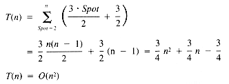
If it is assumed that Target is as likely to be one value (see section 1.3.1) in the range 1 . . Spot as another, then the expected value of Target is
whence:
It is possible to speed up the Find process with a search technique called binary search, which will be discussed in section 7.3. Binary search will not change the order of InsertionSort, however, because the repeated use of Shift forces InsertionSort to be an O(n2) algorithm anyway. The Shift operation can be avoided with a data structure, the linked list, which will be discussed in Chapter 3. The use of a linked list, however, precludes the use of a binary search, so the Find operation is relatively slow.
One might be tempted to conclude that sorting algorithms are all O(n2) or larger. The proof of statements of this type is part of the theory of algorithms. The correct statement is that sorting algorithms are at least of the order n
Exercise E1.4 is appropriate at this point. Programs PGA.1 and PGA.2 and project PJA.1 (See Part II, section A of this book.) are appropriate but depend on familiarity with the material in Part II, section A.
Computing systems, the programs to which they are applied, and the systems that motivate creation of the programs all tend to increase in complexity as computer science matures. They frequently cannot be characterized by analytical means. One consequence is the growing realization that the behavior of these systems and of even relatively simple programs should be studied experimentally. In practice, that involves choosing from distributions with a pseudorandom number generator and applying statistical measures to results. A very brief introduction to tools that can be used for this kind of study is to be found in Part II, section A.
Programming beyond the elementary level requires knowledge, analysis, and technique. Data structures are an essential part of the knowledge, analysis at some level is needed to compare algorithms, and technique comes with practice and with the awareness of possible variations.
Pseudocode provides a language-independent medium for expressing algorithms. One form (SUE) closely tied to Pascal and similar languages is introduced here.
An introduction to the timing of algorithms leads to the determination of the order of growth by summation or inspection. The growth behavior of algorithms provides a measure of comparison for them throughout the book. The discussion in this chapter is background for understanding the assignment of orders of growth. The timing of three basic sorting algorithms provides an example of the top-down summation approach to deriving timing functions.
A brief discussion of random processes is provided in Part II, section A, as an indication of how the average-case behavior of algorithms and the experimental approach to investigating programs can be carried out. This material is optional and left to program assignments.
variable
 expression Assignment. The keystrokes that form the
 assignment operator are a matter of syntax.
Write(v1,v2, . . . ,vn) Output the values of a list of variables or
messages. (The distinctions between Write
and Writeln in Pascal, and between the
effects of commas and semicolons in BASIC,
are features of specific languages.)
Read(v1,v2, . . . ,vn) Input the values of a list of variables. This
form, and Write, will also serve for files
when v1 is a file identifier.
if condition S1 and S2 may be any sequence of
then S1 statements. The else phrase may be missing. In
else S2 a nested structure, an else phrase is taken to
endif be part of the most recent if.
if A < B
then if A < C
then Write(C)
else Write(A)
endif
endif
case The conditions condi must be TRUE or
cond1: S1 FALSE. Si can be any sequence of
cond2: S2 statements, and will be executed iff (if and only
. if) condi is TRUE. It is the programmer's
. responsibility to make sure that only one
. condition can be TRUE; there should be no
condn: Sn overlap. The else may be omitted, in which
else: Se case if no condi is TRUE, then no execution
endcase will take place in this statement.
case of V Here the variable V must take on discrete
Value1: S1 values. It is sometimes convenient to use
Value2: S2 values such as Small, Medium,
. Large--instead of, for example, 1,2,3--although many
. languages do not support this feature. A
. language that restricts case values to be
Valuen: Sn ordinal (ordered discrete), may require a table
else: Se lookup or other map for implementation.
endcase
repeat Here S1 and S2 may be any sequence of
S1 statements. The test for exit is in the middle,
if cond then exit endif not at the top or at the bottom. The
S2 condition must be TRUE or FALSE. The exit
forever passes control to [next statement].
[next statement]
Pascal SUE
REPEAT repeat
Read(x); Read(x)
IF x < O THEN GOTO 1; if x < 0 then exit endif
Sum := Sum + x Sum
 Sum + x
 UNTIL Sum > 100; until Sum > 100
1 : Write (Sum) Write(Sum)
repeat The condition cond must be TRUE or
S FALSE. S is any sequence of statements.
until cond The test for exit occurs explicitly at the
bottom, thus S will be executed at least once.
S may include an exit.
while cond do The condition cond must be TRUE or
S FALSE. S is any sequence of statements.
endwhile The test for exit occurs explicitly at the
top, thus S may not be executed at all. S may
include an exit.
for v = Init to Final by Step do S is any sequence of statements. The
S next v may be replaced by endfor if
next v convenient. The by Step part is
omitted when the Step value is 1. The
use of downto and a negative step
value will run thae count from high
to low.
v
 Init Init, Final, and Step may be expressions,
while v
 Final do and the control values derived from them on
 S entry to the loop do not change during loop
v
 v + Step execution. This is true even if they are
 endwhile variables that have assignments made to them
within the loop. The expression Step may be
negative, in which case the test for exit
becomes while v >= Final do.
1.2.1 Subprograms
procedure Main procedure AddAbs(v)
. if v < 0
. then Sum
 Sum - v
 . else Sum
 Sum + v
 Sum
 0 endif
 AddAbs(x) end {AddAbs Read(y)
AddAbs(y)
Write(Sum)
.
.
.
end {Mainprocedure Main function Abs(v)
. if v < 0
. then Abs
 -v
-v . else Abs
 v
v Sum
 0 endif
 Sum
 Sum + Abs(x) end {Abs
 Read(y)
Sum
 Sum + Abs(y)
 Write(Sum)
.
.
.
end {MainPascal SUE
FUNCTION Min(m,n : REAL): REAL; function Min(m,n)
LABEL 1;
BEGIN
IF (m < 0) AND (n < 0) if (m < 0) AND (n < 0)
THEN BEGIN then return 0
Min := 0;
GOTO 1 endif
END; if m > n
IF m > n then return n
THEN Min := n else return m
ELSE Min := m; endif
1 : END; end {Min1.2.2 Records and Pointers


 Nodule.
 is itself an identifier xNode, and there may not be a need for a variable xNode. The value of x is the address of xNode. This is pictorially represented by:
 Nodule. When p is a pointer of type
  Nodule, then NEW(p) will be assumed to have the effect
 .
.1.3 The Timing of Algorithms
[statement 1]
for i = 1 to n do
[statement 2]
[statement 3]
next i
T(n) = 1 + 2n
T(n) = t1 + (t2 + t3)n
[statement 2]: for j = 1 to m do
[statement 4]
next j {t2 = m  t4
t4[statement 2]: for j = 1 to i do
[statement 4]
next j
Now we have, since m = i:


program TrailMin
Read(Entry[1])
Mindex
 1
1for i = 2 to n do
Read(Entry[i])
if Entry [i] < Entry[Mindex]
then Mindex
 i
iendif
next i
for i = Mindex + 1 to n do
Write(Entry[i])
next i
end {TrailMin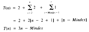
 n + b, a linear function of n.
1.3.1 The Order of Growth
Table 1.1


 n + b will be overtaken, passed, and left in the dust eventually, by any quadratic function TQ(n) = c
  n2 + d
  n + e. This happens no matter what the values of a, b, c, d, and e may be. The crucial factor, for a polynomial, is the highest power of n.
 c|g(n)| for all n > m.
 n + b = O(n). A proof of this is:


[statement 1]
for i = 1 to n do
[statement 2]
[statement 3]
next i
1.3.2 The Variability of Data (optional)



1.4 Comparison of Three Sorts (optional)
program InOut(n)
Ingress(n) {Input n entries into array e.Sort(n) {Arrange the entry values in nondecreasing order.OutHaul(n) {Display e in (its new) order.end {InOutprocedure Ingress(n) {O(n)for i = 1 to n do
Read(e[i])
next i
end {Ingressprocedure OutHaul(n) {O(n)for i = 1 to n do
Write(e[i])
next i
end {OutHaul1.4.1 SelectionSort (optional)

Figure 1.1
 Target. This determines an index, Spot, of that maximal value. The exchange is made with e[Target] and e[Spot].
procedure SelectionSort(n)
for Target = 1 to n - 1 do
Large
 e[Target]
Spot
 Target
Hun {For the index, Spot, of a maximal {value among the remaining entries.Temp
 e[Spot]
e[Spot]
 e[Target]
e[Target]
 Temp
Tempnext Target
end {SelectionSort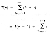
procedure Hunt
for i = Target + 1 to n do
if e[i] > Large
then Spot
 i
iLarge
 e[Spot]
endif
next i
end {Hunt
1.4.2 BubbleSort (optional)
-5 2 10 -7 0 10

Figure 1.2
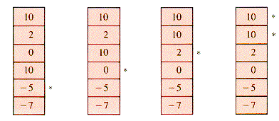
Figure 1.3
procedure BubbleSort(n)
for Target = n downto 2 do
Slide(Target) {smallest-so-far into e[Target]next Target
end {BubbleSort
procedure Slide(Target)
for i = 1 to Target - 1 do
if e[i] < e[i +1]
then Temp
 e[i]
e[i]e[i]
 e[i + 1]
e[i + 1]
 Temp
Tempendif
next i
end {Slide
1.4.3 InsertionSort (optional)

Figure 1.4
 j
j  i}, where e[i] should be placed. If j < i, the values e[j], e[j+1], . . . for k = Target to (i - 1) need to be shifted out of the way. Finally, the old value of e[i] is assigned to e[Target]. This becomes:
procedure InsertionSort(n)
for Spot = 2 to n do
Find(Target,Spot)
Temp
 e[Spot]
Shift(Target, Spot)
e[Target]
 Temp
Tempnext Spot
end {InsertionSort
procedure Find(Target,Spot) {f = 1 + (Spot - 1)Target
 Spot
Spotfor i = 1 to Spot - 1 do { = Spotif e[i] < e[Spot]
then Target
 i
iexit
endif
next i
end {Findprocedure Shift(Target,Spot)
for i = Spot downto Target + 1 do
e[i]
 e[i - 1]
next i {s = Spot - Targetend {Shift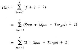

 ln n. The sorting problem itself is intrinsically O(n . ln n), no matter what algorithms are dreamed up to solve it. Sorting algorithms that have O(n
  ln n) behavior are discussed in Chapters 8 and 9.
1.5 Random Processes (optional)
Summary


